import matplotlib.pyplot as plt
import numpy as np
Define Test Function and Derivatives¶
Let’s get started by defining a test function we will use throughout the notebook.
Consider a scalar function to allow for easier visualization. Let
## Define f(x)
f = lambda x: 0.5 * (x - 1) ** 4 + (x + 1) ** 3 - 10 * x**2 + 5 * x

## Define f'(x)
df = lambda x: 6 - 8 * x - 3 * x**2 + 2 * x**3

## Define f''(x)
ddf = lambda x: -8 - 6 * x + 6 * x**2
plt.figure()
xplt = np.arange(-3, 4, 0.1)
fplt = f(xplt)
dfplt = df(xplt)
ddfplt = ddf(xplt)
# House cycle in order (figures/dowling.mplstyle): black solid, blue dashed,
# orange dash-dot. These were matplotlib's "b"/"r"/"g", which are outside the
# Okabe-Ito palette the rest of the notebook now uses.
plt.plot(xplt, fplt, label="f(x)", color="black", linestyle="-")
plt.plot(xplt, dfplt, label="f'(x)", color="#0072B2", linestyle="--")
plt.plot(xplt, ddfplt, label="f''(x)", color="#E69F00", linestyle="-.")
plt.xlabel("x")
plt.legend()
plt.grid()
plt.show()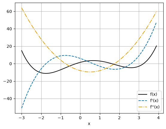
Geometric Insights into Newton Steps¶
Motivation¶
We can interpret Newton-type methods for unconstrained optimization as root finding of .
At iteration , we assemble an approximation to using a Taylor series expansion:
Set the gradient of this quadratic model to zero, . For nonsingular , the resulting linear solve gives:
The choice of determines the algorithm classification:
Pure Newton Method,
Steepest Descent, , where scalar is sometimes known as the dampening factor
Levenberg-Marquardt, , where scalar is chosen to ensure is positive definite.
Broyden Methods, is approximated using history of gradient evaluations, i.e., . We will study the SR1 and BFGS formulas in this family of methods.
This section explores how choosing impacts the shape of the approximation and calculated step.
Compute and Plot Steps¶
Define a function that:
Computes the i. Newton, ii. Levenberg-Marquardt and iii. Steepest Descent Step for a given starting point
Plots the step in terms of and
def calc_step(x0, epsLM):

    # Evaluate f(x0), f'(x0) and f''(x0)
    f0 = f(x0)
    df0 = df(x0)
    ddf0 = ddf(x0)
    print("x0 = ", x0)
    print("f(x0) =", f0)
    print("f'(x0) =", df0)
    print("f''(x0) =", ddf0)

    ### Calculate steps

    # Newton Step
    xN = x0 - df0 / ddf0

    print("\n### Newton Step ###")
    print("xN = ", xN)
    print("pN = xN - x0 = ", xN - x0)
    f_xN = f(xN)
    print("f(xN) = ", f_xN)
    print("f(xN) - f(x0) = ", f_xN - f0)

    # Levenberg-Marquardt Step
    # Recall the eigenvalue of a 1x1 matrix is just that value
    dffLM = np.amax([ddf0, epsLM])
    xLM = x0 - df0 / dffLM

    print("\n### Levenberg-Marquardt Step ###")
    print("xLM = ", xLM)
    print("pLM = xLM - x0 = ", xLM - x0)
    f_xLM = f(xLM)
    print("f(xLM) = ", f_xLM)
    print("f(xLM) - f(x0) = ", f_xLM - f0)

    # Steepest Descent Step
    xSD = x0 - df0 / 1

    print("\n### Steepest Descent Step ###")
    print("xSD = ", xSD)
    print("pSD = xSD - x0 = ", xSD - x0)
    f_xSD = f(xSD)
    print("f(xSD) = ", f_xSD)
    print("f(xSD) - f(x0) = ", f_xSD - f0)

    ### Plot Surrogates on x vs f(x)

    ### Plot f(x)
    # Okabe-Ito colors paired with distinct linestyles and markers, in the
    # order used by figures/dowling.mplstyle: black solid, blue dashed, orange
    # dash-dot, bluish green dotted. All three surrogates used to be dashed and
    # were told apart by color alone, which does not survive a photocopy.
    plt.figure()
    plt.scatter(x0, f0, label="$x_0$", color="black", zorder=5)
    plt.plot(xplt, fplt, label="f(x)", color="black", linestyle="-")

    ### Plot approximation for Newton's method
    fN = lambda x: f0 + df0 * (x - x0) + 0.5 * ddf0 * (x - x0) ** 2
    plt.plot(xplt, fN(xplt), label="Newton", linestyle="--", color="#0072B2")
    plt.scatter(xN, f(xN), color="#0072B2", marker="x")

    ### Plot approximation for LM
    fLM = lambda x: f0 + df0 * (x - x0) + 0.5 * dffLM * (x - x0) ** 2
    plt.plot(xplt, fLM(xplt), label="LM", linestyle="-.", color="#E69F00")
    plt.scatter(xLM, f(xLM), color="#E69F00", marker="s")

    ### Plot approximation for SD
    fSD = lambda x: f0 + df0 * (x - x0) + 0.5 * (x - x0) ** 2
    plt.plot(xplt, fSD(xplt), label="Steepest", linestyle=":", color="#009E73")
    plt.scatter(xSD, f(xSD), color="#009E73", marker="^")

    # plt.plot([x0, xLM],[f0, f(xLM)],label="LM",color="green",marker="o")
    # plt.plot([x0,xSD],[f0,f(xSD)],label="Steepest",color="blue",marker="s")

    plt.xlim((-3.5, 4.5))
    plt.ylim((-12.5, 22.5))
    plt.xlabel("$x$")
    plt.ylabel("$f(x)$")
    plt.legend()
    plt.title("Function and Surrogates")
    plt.grid()
    plt.show()

    ### Plot Surrogates on x vs f'(x)
    plt.figure()
    plt.scatter(x0, df0, label="$x_0$", color="black", zorder=5)
    plt.plot(xplt, dfplt, label="f'(x)", color="black", linestyle="-")

    ### Plot approximation for Newton's method
    dfN = lambda x: df0 + ddf0 * (x - x0)
    plt.plot(xplt, dfN(xplt), label="Newton", linestyle="--", color="#0072B2")
    plt.scatter(xN, df(xN), color="#0072B2", marker="x")

    ### Plot approximation for LM
    dfLM = lambda x: df0 + dffLM * (x - x0)
    plt.plot(xplt, dfLM(xplt), label="LM", linestyle="-.", color="#E69F00")
    plt.scatter(xLM, df(xLM), color="#E69F00", marker="s")

    ### Plot approximation for SD
    dfSD = lambda x: df0 + (x - x0)
    plt.plot(xplt, dfSD(xplt), label="Steepest", linestyle=":", color="#009E73")
    plt.scatter(xSD, df(xSD), color="#009E73", marker="^")

    plt.xlim((-3.5, 4.5))
    plt.ylim((-50, 50))
    plt.xlabel("$x$")
    plt.ylabel("$f'(x)$")
    plt.legend()
    plt.title("First Derivative and Surrogates")
    plt.grid()
    plt.show()
Consider ¶
calc_step(-3, 1e-2)x0 = -3
f(x0) = 15.0
f'(x0) = -51
f''(x0) = 64
### Newton Step ###
xN = -2.203125
pN = xN - x0 = 0.796875
f(xN) = -8.660857647657394
f(xN) - f(x0) = -23.660857647657394
### Levenberg-Marquardt Step ###
xLM = -2.203125
pLM = xLM - x0 = 0.796875
f(xLM) = -8.660857647657394
f(xLM) - f(x0) = -23.660857647657394
### Steepest Descent Step ###
xSD = 48.0
pSD = xSD - x0 = 51.0
f(xSD) = 2534689.5
f(xSD) - f(x0) = 2534674.5
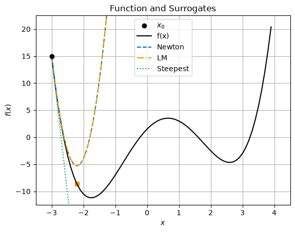
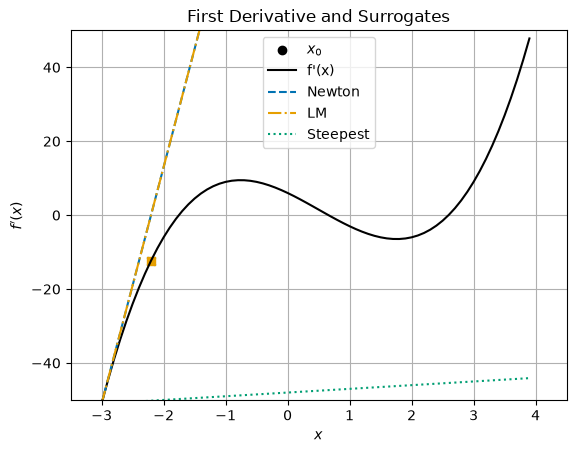
Discussion
In this case, do we expect the Newton and LM steps to be the same? Explain.
Why does increase with a steepest descent () step? I thought the main idea was that because is positive definite the step is in a descent direction!
Consider ¶
calc_step(0, 1e-2)x0 = 0
f(x0) = 1.5
f'(x0) = 6
f''(x0) = -8
### Newton Step ###
xN = 0.75
pN = xN - x0 = 0.75
f(xN) = 3.486328125
f(xN) - f(x0) = 1.986328125
### Levenberg-Marquardt Step ###
xLM = -600.0
pLM = xLM - x0 = -600.0
f(xLM) = 65014556401.5
f(xLM) - f(x0) = 65014556400.0
### Steepest Descent Step ###
xSD = -6.0
pSD = xSD - x0 = -6.0
f(xSD) = 685.5
f(xSD) - f(x0) = 684.0
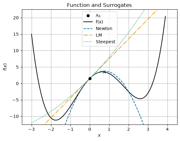
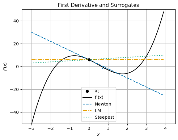
Discussion
Why does increase for all of the steps?
Explain Newton-type method in the context of root finding for using the second plot.
Descent Properties¶
For , positive definiteness of gives
Thus is a descent direction whenever . A line search still chooses a step length that produces sufficient decrease. (Biegler, Eqs. 3.2--3.5, p. 41.)
Line Search¶
Excerpts from Section 3.4 in Biegler (2010).
Sufficient decrease and curvature conditions¶
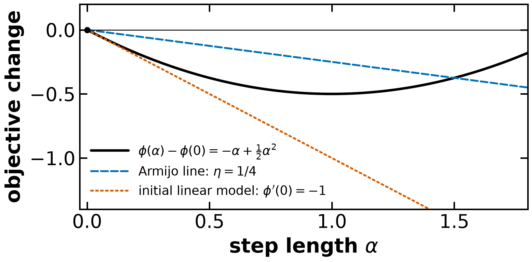
Let on an open , with . At a fixed direction, define and . For fixed , the Armijo condition for a feasible positive length is
Here feasible means that the trial point lies in the objective domain. The condition requires a fraction of the initial linear-model decrease. Since , sufficiently short positive steps pass. It also permits unnecessarily small steps if the selection rule has no lower-size control.
Use for the Goldstein--Armijo conditions, which add the lower value bound:
Near zero the actual curve initially drops faster than the lower line, so that line excludes very short steps. For the profile , , the positive accepted interval is .
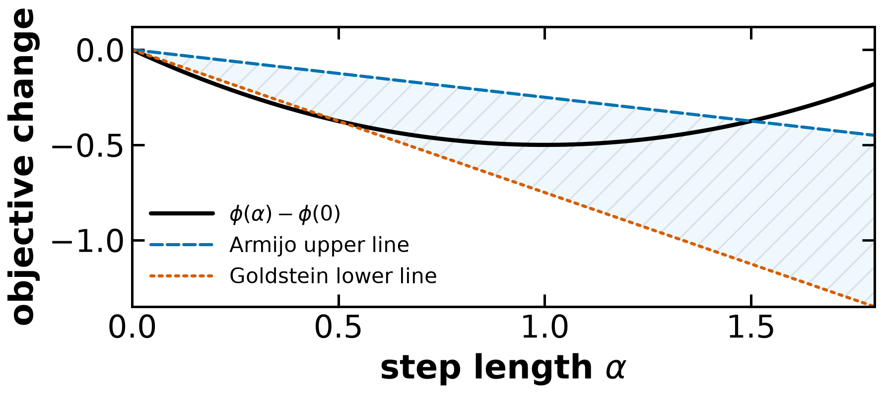
Alternatively, choose . Wolfe combines Armijo with ; strong Wolfe combines it with . These require a directional derivative at a trial point. Goldstein uses function values. On a nonconvex ray the accepted set need not be one connected interval; the brackets in a particular figure describe that example.
Sources: Biegler (2010), Eqs. (3.31)--(3.34), pp. 47--48, with the ordering correction in the errata; Nocedal and Wright (2006), Eqs. (3.4), (3.6)--(3.7), (3.11), pp. 33--36. The general Armijo range is ; the strict choice also supplies the margin used in the unit-step result below.
Global convergence: gradient norms and the descent angle¶
Use Euclidean vector norms and their induced matrix norm. Consider a nonterminated sequence of descent steps, with bounded below and continuously differentiable, and its gradient uniformly Lipschitz on an open set containing the initial sublevel set. Lipschitz continuity means that some satisfies for every pair in that open set. The acceptance parameters are fixed across the sequence. Write
For Goldstein--Armijo steps, the Zoutendijk sum is finite:
Here is the value-based proof. Fix an iteration and let be the first positive crossing of the Goldstein lower line before the accepted . Such a crossing exists because the curve starts below that line and the accepted value lies at or above it. On , the curve lies below that line and therefore within the initial sublevel set. The gradient Lipschitz bound gives
At the crossing the left side is , so
Armijo now supplies
Summing telescopes the actual decreases, and has a lower bound. The resulting sum is finite. Biegler’s mean-value proof uses a looser constant; the conclusion is the same. A Wolfe proof instead compares the directional derivatives at the two endpoints, yielding the analogous Zoutendijk result.
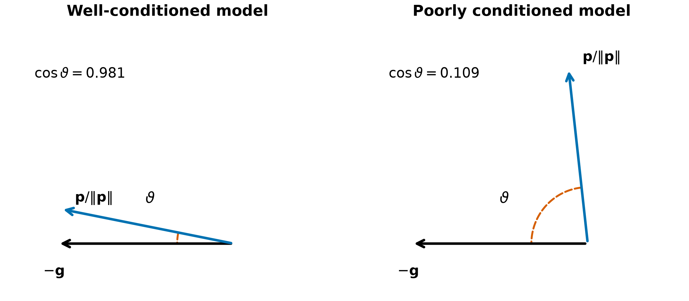
For , with symmetric ,
A uniform condition-number bound therefore forces . Every accumulation point is stationary by gradient continuity. This does not by itself prove convergence of the whole iterate sequence, second-order conditions, or global optimality.
Sources: Biegler (2010), Theorem 3.3 and Eqs. (3.35)--(3.42), pp. 48--49; Nocedal and Wright (2006), Theorem 3.2, p. 38, for Wolfe steps. The eigenvalue/norm estimates have their existing home in Quasi-Newton Methods; they are applied here to the search angle.
Armijo backtracking and the actual visualization code¶
The standard reference procedure starts with a descent direction, tries , and, while Armijo fails, replaces by , with fixed . It accepts the first trial that passes Armijo. The local argument above ensures finite termination along a descent ray. The previous rejected trial prevents uncontrolled overshrinking by the selection rule. If contractions vary, safeguard them between fixed positive lower and upper bounds below one.
This is not a rule to keep shrinking until both Goldstein bounds pass. For , , Goldstein--Armijo accepts . Halving from one first passes Armijo at . A contraction by 10-3 jumps to 0.001, below the Goldstein interval; every further contraction remains below it. To require Goldstein or Wolfe, use a suitable bracketing/selection method that can increase a trial when the lower-size test fails.
The function plot_alpha below is a graphical experiment: it evaluates a finite, linearly spaced grid, scans it downward, exempts its initial full trial from the Goldstein check, and reports a lower-bound failure on later trials. It is not the geometric backtracking algorithm just stated or a general Wolfe solver. Its deliberate ascent-direction and restricted-grid failures remain part of the exercise.
A condition-number bound alone is sufficient in the Goldstein theorem above, but is not sufficient for a unit-step-capped Armijo method: directions can shrink summably even with condition number one. A conventional global Armijo result also controls the scale of the direction, for example by uniform positive lower and upper eigenvalue bounds on .
Sources: Nocedal and Wright (2006), Algorithm 3.1 and discussion, p. 37; Dennis and Schnabel (1996), Algorithm 6.3.5, p. 126; Biegler (2010), Algorithm 3.2 and the additional Goldstein discussion, p. 50. Safeguarded quadratic/cubic interpolation is detailed below.
Recovery of the fast local rate¶
Suppose on an open neighborhood of the limit, and a nonterminated descent sequence with nonzero directions converges to , , and . Use fixed Wolfe parameters and . Let the directions satisfy
For Newton-type solves this is the Dennis--Moré directional condition. Nondegeneracy and the residual condition imply . They also give eventually, for some .
Taylor expansion and the small residual give
Thus Armijo has negative slack when ; the curvature condition also passes for fixed . Unit steps are eventually admissible. The search must try and accept them to obtain the superlinear rate. Admissibility alone does not force that selection.
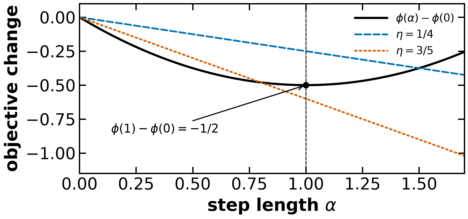
The endpoint has no Taylor-error margin. For , near zero, exact Newton gives . Its unit step fails endpoint Armijo, but its half step satisfies Wolfe with for sufficiently small negative . The half-step recurrence is
It stays negative near zero and converges only linearly despite zero Newton directional residual. We therefore use the conservative strict parameter bound in the handout/reference. The whole-iterate versus directional-error equivalence has its existing full proof in Quasi-Newton Methods; the local Newton error proof is in Newton Methods.
Sources: Nocedal and Wright (2006), Theorems 3.6--3.7, pp. 46--47; Biegler (2010), Theorem 3.4, p. 50, with nondegeneracy explicit. The endpoint example is an independently derived illustration.
Visualization Code¶
The line search conditions, as one picture¶
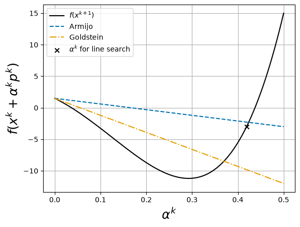
![Armijo and Goldstein conditions for steepest descent from x^k=-3: the accepted step lengths are the interval [\alpha_g, \alpha_a] where the function value stays below the Armijo line and above the Goldstein line.](/optimization/build/eb19b57463aecb83e9e175e2d11e404f.png)
This is Biegler Figure 3.2 for our test function. It is rendered from
figures/plots/line-search-conditions.py and is the same image printed in the course
pack, so what you annotate in lecture and what you see here cannot drift apart.
The cells below are the live version: plot_alpha redraws this for any , any
algorithm and any , so you can explore cases the static figure does not
cover -- including one where the line search fails.
Goal: Visualize Armijo and Goldstein conditions for an example.
def plot_alpha(xk, eta_ls=0.25, algorithm="newton", alpha_max=1.0):
    """
    Calculate step and visualize line search conditions

    Arguments:
        xk : initial point (required)
        eta_ls : eta in Goldstein-Armijo conditions
        algorithm : either "newton" or "steepest-descent"
        alpha_max : plots alpha between 0 and alpha_max

    Returns:
        Nothing

    Creates:
        Plot showing function value and line search conditions as a function of alpha
    """

    fxk = f(xk)
    dfxk = df(xk)

    if algorithm == "newton":
        pk = -dfxk / ddf(xk)
    elif algorithm == "steepest-descent":
        pk = -dfxk
    else:
        raise ValueError(
            "algorithm argument must be either 'newton' or 'steepest-descent'"
        )

    print("Considering xk =", xk, "and f(xk) = ", fxk)
    print("Step with", algorithm, "algorithm:")
    print("pk = ", pk)
    print("With full step, xk+1 =", pk + xk, "and f(xk+1) =", f(xk + pk))

    n = 100
    alpha = np.linspace(0, alpha_max, n)
    fval = np.zeros(n)

    for i in range(0, n):
        fval[i] = f(xk + alpha[i] * pk)

    fs = 18
    plt.figure()

    # Evaluate f(x^{k+1}) for different alpha values.
    # Color and linestyle match figures/plots/line-search-conditions.py, the
    # static version of this figure in the course pack: house cycle in order,
    # black solid, blue dashed, orange dash-dot. The linestyles are what make
    # the three series separable in greyscale.
    plt.plot(alpha, fval, color="black", linestyle="-", label=r"$f(x^{k+1})$")

    # Armijo condition
    arm = np.zeros(n)
    for i in range(0, n):
        arm[i] = fxk + eta_ls * alpha[i] * dfxk * pk

    plt.plot(alpha, arm, color="#0072B2", linestyle="--", label="Armijo")

    # Goldstein condition
    gold = np.zeros(n)
    for i in range(0, n):
        gold[i] = fxk + (1 - eta_ls) * alpha[i] * dfxk * pk

    plt.plot(alpha, gold, color="#E69F00", linestyle="-.", label="Goldstein")

    # Apply backtracking linestep (starting with alpha = alpha_max)
    i = n - 1
    flag = True
    failed = False
    while flag:

        if i < n - 1 and fval[i] < gold[i]:
            flag = False
            print(
                "Line search failed. Goldstein conditions violated. Consider increasing alpha_max."
            )
            failed = True

        # Armijo condition
        if fval[i] < arm[i]:
            flag = False
        else:
            i = i - 1

        if i < 0:
            print("Line search failed. Try decreasing alpha_max.")
            failed = True
            # Stop here. Without this, the loop keeps going with a negative
            # index, which wraps around to the end of the array and reports a
            # second, contradictory diagnosis.
            flag = False

    if not failed:
        print(
            "alphak =",
            alpha[i],
            "with backtracking line search starting at alpha =",
            alpha_max,
        )
        print("f(xk + alphak*pk) =", fval[i])

        plt.scatter(
            alpha[i],
            fval[i],
            marker="x",
            color="black",
            label=r"$\alpha^{k}$ for line search",
        )

    # Labels
    plt.xlabel(r"$\alpha^k$", fontsize=fs)
    plt.ylabel(r"$f(x^k + \alpha^k p^k)$", fontsize=fs)
    plt.grid()
    plt.legend()
    plt.show()
Newton Step, ¶
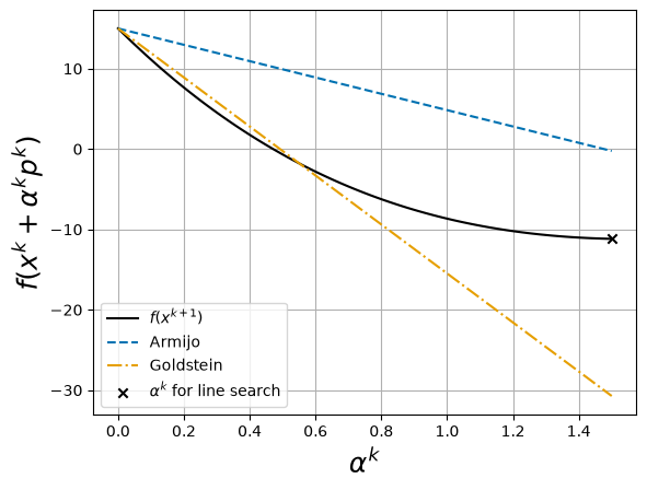
plot_alpha(-3, eta_ls=0.25, algorithm="newton", alpha_max=1.5)Considering xk = -3 and f(xk) = 15.0
Step with newton algorithm:
pk = 0.796875
With full step, xk+1 = -2.203125 and f(xk+1) = -8.660857647657394
alphak = 1.5 with backtracking line search starting at alpha = 1.5
f(xk + alphak*pk) = -11.1743426900357
Discussion
Why did the backtracking line search stop at
alpha_max?Is it possible to find a larger improvement in with ?
Steepest Descent Step, ¶
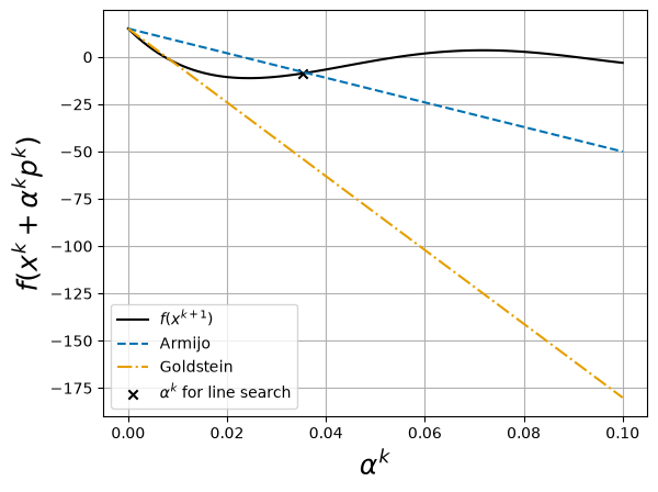
plot_alpha(-3, eta_ls=0.25, algorithm="steepest-descent", alpha_max=1e-1)Considering xk = -3 and f(xk) = 15.0
Step with steepest-descent algorithm:
pk = 51
With full step, xk+1 = 48 and f(xk+1) = 2534689.5
alphak = 0.03535353535353535 with backtracking line search starting at alpha = 0.1
f(xk + alphak*pk) = -8.67145500733185
Discussion
Why did the line search stop where the Armijo conditions are satisfied?
Why not further decrease to achieve a greater improvement in the objective?
Newton Step, ¶
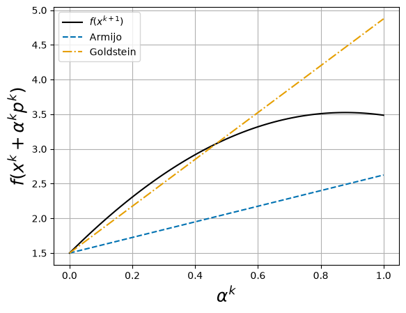
plot_alpha(0, eta_ls=0.25, algorithm="newton", alpha_max=1.0)Considering xk = 0 and f(xk) = 1.5
Step with newton algorithm:
pk = 0.75
With full step, xk+1 = 0.75 and f(xk+1) = 3.486328125
Line search failed. Goldstein conditions violated. Consider increasing alpha_max.
Discussion
Why does the line search fail?
How could we modify Newton’s method to improve robustness?
Steepest Descent Step, ¶
plot_alpha(0, eta_ls=0.25, algorithm="steepest-descent", alpha_max=5e-1)Considering xk = 0 and f(xk) = 1.5
Step with steepest-descent algorithm:
pk = -6
With full step, xk+1 = -6 and f(xk+1) = 685.5
alphak = 0.4191919191919192 with backtracking line search starting at alpha = 0.5
f(xk + alphak*pk) = -2.9749848430038526
Discussion
How does the region where the Armijo and Goldstein conditions are satisfied change for different values of
eta_ls?
Trust Regions¶
Excerpts from Section 3.5 in Biegler (2010).
Main Idea and General Algorithm¶
At iteration , with , the closed ball is . A line search instead restricts its nonzero fixed direction to . With symmetric , use the Euclidean-ball subproblem
The constant is omitted because it changes neither the minimizer nor the predicted reduction. Weierstrass states that a continuous function on a nonempty compact set attains its minimum and maximum; its existing existence discussion is in Unconstrained Optimality Conditions. A continuous quadratic therefore attains a minimum on this compact ball even when is indefinite.
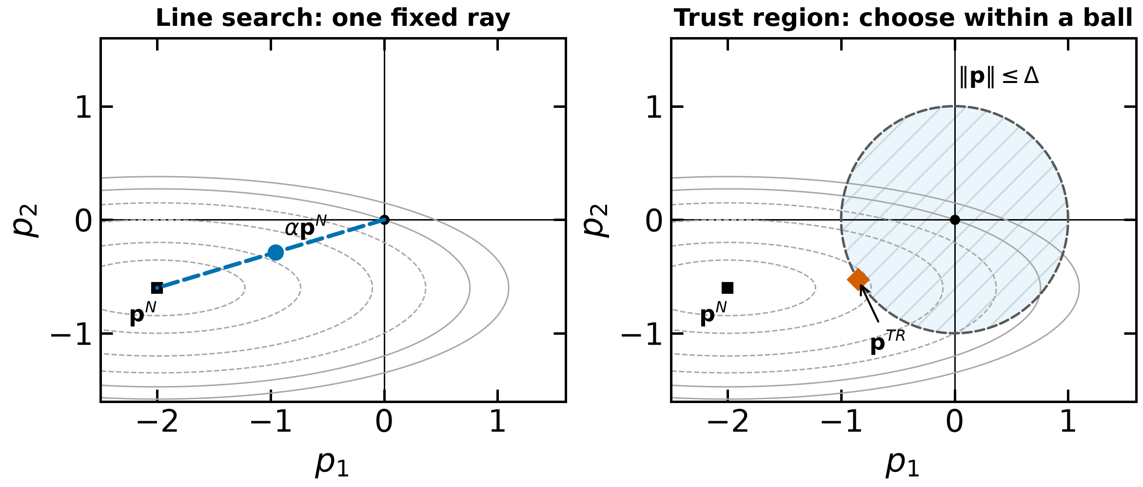
The radius is updated by comparing actual objective reduction with predicted model reduction. Source: Biegler (2010), Eq. (3.49), p. 53; Nocedal and Wright (2006), pp. 68--70.
Choose , , and . Evaluate the current gradient before testing it; a small gradient reports a stationary candidate. For a nonterminated iteration:
Compute a feasible, sufficiently model-reducing step . Report stagnation together with the gradient norm if its movement is too small.
Compute . A nonpositive prediction signals a failed subproblem step; do not form a meaningless ratio.
Evaluate and .
If , set . If and the step reaches the boundary, set . Otherwise retain the radius.
Accept the trial iterate only if ; otherwise retain the old iterate and recompute a step with the new radius.
Acceptance and radius change have different thresholds. With prediction 10, actual decrease 1.5, , , and step norm 2, the ratio is 0.15: accept the step but shrink the next radius to 0.5. A good interior step need not enlarge the radius because the current bound did not restrict it.
Source: Biegler (2010), Algorithm 3.3, p. 53, adapted to test evaluated quantities and report failed diagnostics. Nocedal and Wright’s Algorithm 4.1, p. 69, uses the closely related shrink rule , rather than Biegler’s step-norm rule; do not silently mix the two.
Why order the thresholds? Every rejected trial has , so it triggers a radius decrease. The strict inequality also handles . Biegler’s usual choice with has this property. His more general parameter list in Algorithm 3.3 does not explicitly state the ordering; the following independently derived example shows why that broader list needs qualification for this update rule.
Consider , starting at , with exact gradient , model curvature , and radius . The exact model minimizer is the interior step , giving
Choose , , and . The trial is rejected because , but the radius is retained because and the expansion condition fails. Reusing the same model repeats the identical rejected step indefinitely, with gradient . The objective is smooth and bounded below, the model matrices are bounded, and the exact step gives sufficient model reduction. Thus those assumptions alone do not establish stationarity when the thresholds allow rejected steps to keep the radius. This example motivates the strict ordering used above; it does not alter the numerical activity’s default parameters.
Trust Region Variations¶
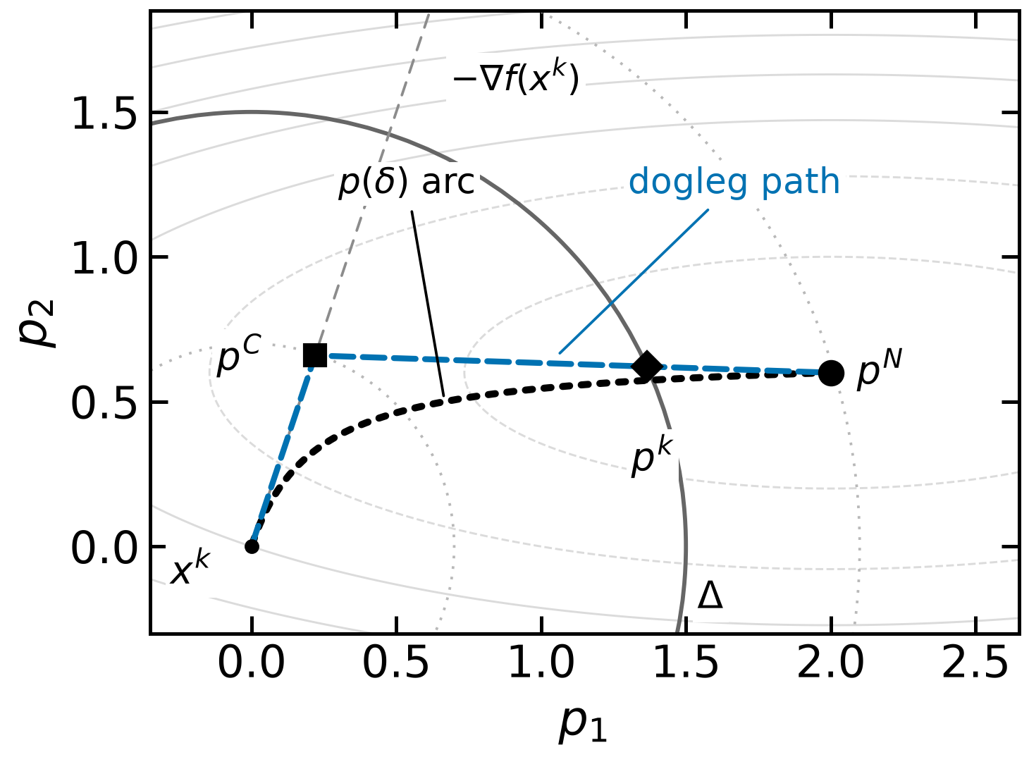
The Levenberg--Marquardt path varies a multiplier continuously; dogleg uses straight segments connecting the origin, Cauchy step, and Newton step.
: Cauchy step
: Newton step
Levenberg-Marquardt¶
Let , , and . A feasible vector is a global minimum of the quadratic model over the ball if and only if some satisfies
Feasibility is essential. If , the boundary is active. The converse fails: a Newton minimum may lie exactly on the boundary with . At a singular shifted matrix, use the linear system and an appropriate null-space component, not an undefined inverse.
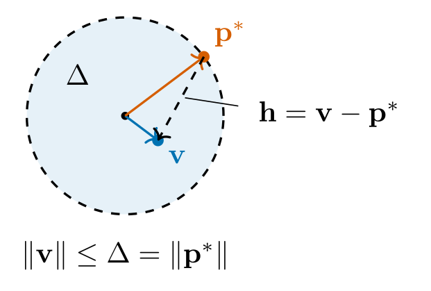
For sufficiency, put , where is any feasible comparison point. Expanding the quadratic and using stationarity yields
The first term is nonnegative by positive semidefiniteness. The second is zero if ; otherwise complementarity puts the candidate on the boundary and feasibility bounds the comparison norm. This certifies the model minimum, not a global minimum of the actual objective. The converse characterization is proved in Nocedal and Wright, pp. 89--91.
Sources: Nocedal and Wright (2006), Theorem 4.1, p. 70; Biegler (2010), Theorem 3.6 and Eq. (3.50), p. 54, with the missing feasibility condition supplied.
Powell Dogleg¶
For , the Cauchy point minimizes the quadratic on the feasible steepest-descent ray. Write . Then
If , the ray model keeps decreasing, so its best feasible point is the boundary. With , the unconstrained ray minimum is used only when it fits. Define that untruncated vector as .
Biegler Eq. (3.52) calls the untruncated positive-curvature vector a Cauchy step and clips it in the later dogleg rule. Nocedal and Wright’s Cauchy point is already clipped. The formulas above distinguish these roles explicitly.
Sources: Biegler (2010), Eq. (3.52), p. 54; Nocedal and Wright (2006), Eqs. (4.11)--(4.12), p. 72.
For , calculate by a solve, and let be the untruncated ray minimum:
If , take the full model minimum.
Otherwise, if , take , the first-leg boundary point.
Otherwise take , where and the second segment intersects the boundary.
The intermediate condition gives . Expanding the norm constraint produces
The applicable root is
This avoids a scalar iteration. In the shared figure, , , and . The inputs give , , and . The dogleg boundary point and the exact L--M boundary point generally differ; the former approximates the full subproblem.
Both norm growth and model decrease along this path rely on positive definiteness. An indefinite exact Hessian needs a method that can use negative curvature, as detailed in the hard-case reference below.
Sources: Biegler (2010), §3.5.1 and Figure 3.4, p. 55; Nocedal and Wright (2006), Eqs. (4.15)--(4.16), p. 74, and Lemma 4.2, p. 75. The generated picture and numerical implementation have one source in the course figure pipeline.
Reference: monotone decrease without stationarity¶
For , , the sequence has decreasing objective values but two limit points, -1 and 1. Its displacement stays large while the actual decrease tends to zero. Let and take . These are descent directions, but their predicted linear decrease has a nonzero asymptotic magnitude. Thus any fixed positive Armijo fraction eventually rejects them.
For , use and . Direct subtraction verifies the recurrence, and the geometric series totals one. The iterates reach the nonstationary limit 1. Actual decrease relative to the initial directional derivative tends to one, so Armijo permits these arbitrarily small steps, while Goldstein or Wolfe eventually rejects them.
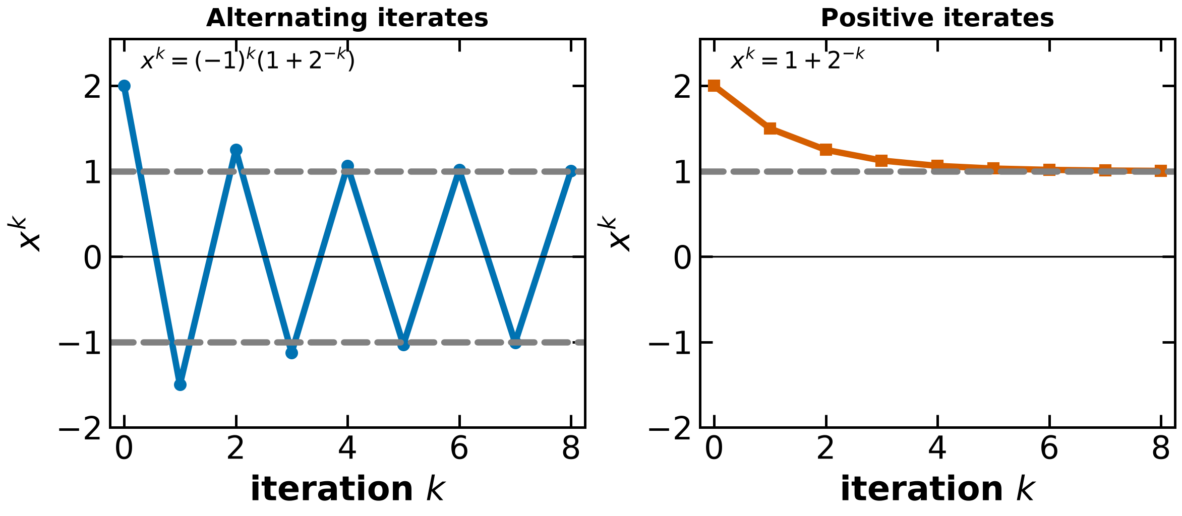
The second exponent corrects the inconsistent printed step sequence in Dennis and Schnabel, p. 118. It follows from subtracting consecutive displayed iterates, rather than adopting an index convention silently.
Sources: Dennis and Schnabel (1996), §6.3 and Figure 6.3.2, pp. 117--118; Biegler (2010), §3.4, pp. 47--48.
Reference: safeguarded interpolation for backtracking¶
Write , , and suppose the positive trial fails Armijo. Fit
If , its minimizer is . This uses only the initial value/slope and one rejected value. If the fit has no useful positive minimum, use a contraction instead.
After two distinct positive rejected trials, define
The cubic fit satisfies both values. Solve , selecting a positive stationary point with positive second derivative. If , use the quadratic formula above; a negative discriminant or unusable minimum calls for fallback.
Do not accept a point merely because it minimizes an interpolant. Safeguard the next trial, for example within , evaluate the actual objective there, and test Armijo again. Safeguards avoid almost unchanged trials and extremely small jumps caused by a poor fit. The two distinct trial values are essential; equal nodes do not define this cubic fit.
A Goldstein/Wolfe search has different lower-size logic: a trial that is too short must be increased or bracketed, not contracted forever. The reference backtracking experiment in the handout with demonstrates this distinction.
Sources: Dennis and Schnabel (1996), §6.3.2, pp. 126--128; Biegler (2010), Algorithm 3.2, p. 50, and Exercise 4, p. 61; Nocedal and Wright (2006), §3.5, pp. 56--60.
Reference: solving the Levenberg--Marquardt secular equation¶
First suppose , , and the Newton model minimum lies outside the radius. For , solve
The norm decreases strictly from its outside value to zero. Solve , preferably via the reciprocal secular function
Differentiating the solve gives . A second solve yields
The same Cholesky factor can serve both solves. Establish a bracket with , increasing the upper trial until it is large enough. A Newton proposal must remain in the admissible bracket; otherwise use a bracketed fallback. Stop at the accuracy appropriate for the model-reduction/feasibility requirement, rather than forcing unnecessary multiplier digits.
The reciprocal form is often nearly linear in the large-shift regime because . Biegler’s two-or-three-iteration observation concerns a useful approximate root; it is not an iteration bound for every model.
For an indefinite matrix, the positive-definite solve domain starts above . A root may fail to exist in that open domain: the hard case requires the singular endpoint and a null-space correction. Repeatedly increasing a shift cannot repair that missing component.
Sources: Biegler (2010), Eq. (3.51), p. 54; Nocedal and Wright (2006), §4.3 and Algorithm 4.3, pp. 85--87.
Reference: Cauchy reduction, stationarity, and collapsing radii¶
For symmetric , , use Euclidean/induced norms and let
This is a feasible ray trial. The quadratic-form norm bound gives
The Cauchy point minimizes over this ray, so its reduction is at least the trial reduction. Any step at least as good as Cauchy therefore supplies
If , the feasible boundary ray gives reduction directly; do not divide by its zero norm. If , first-order stopping/classification is separate, and an indefinite model may still have a negative-curvature reduction.
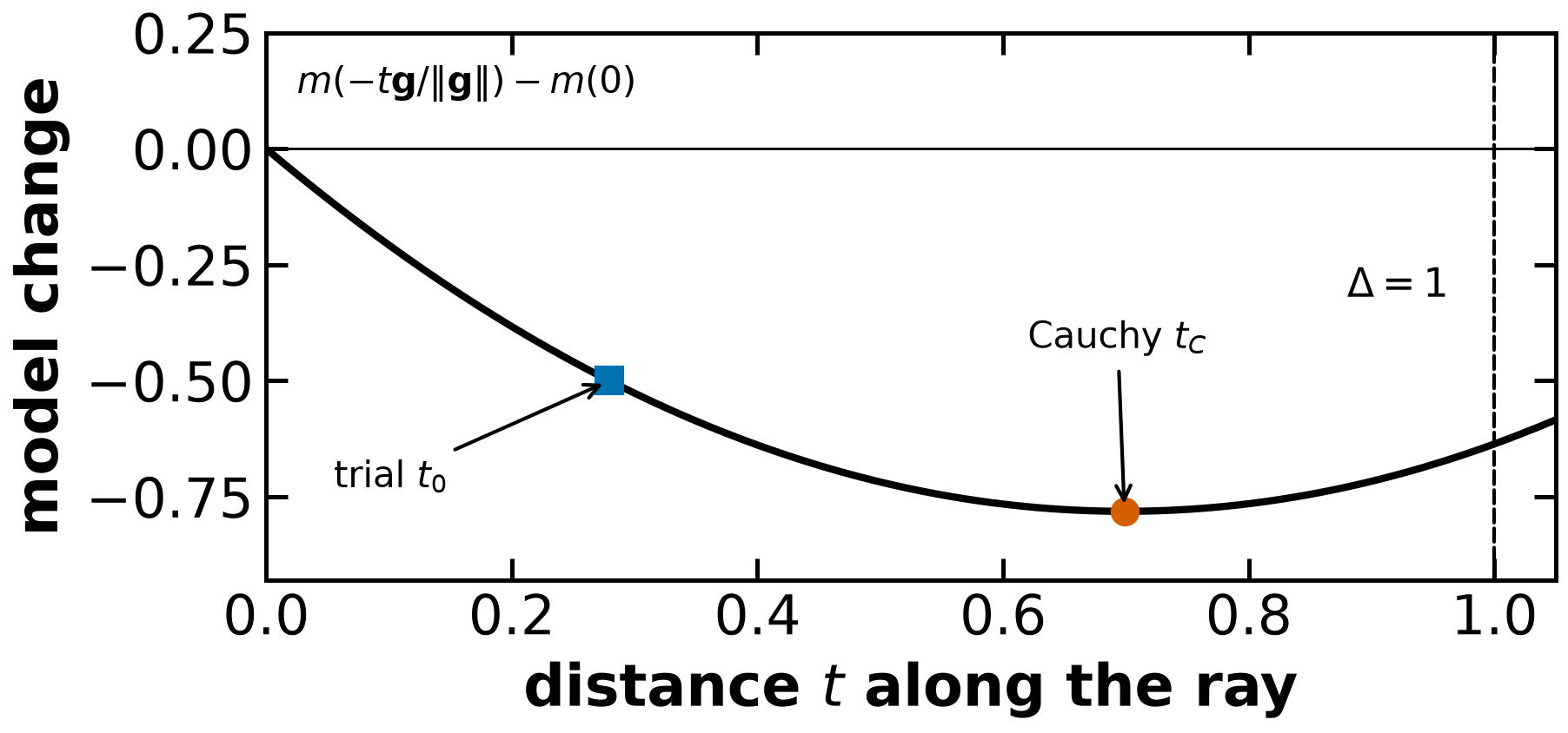
Exact model minima satisfy the bound. Positive-definite dogleg steps do too, because the chosen point is at least as good as the feasible Cauchy point. A fixed positive fraction of this bound is enough in the general convergence framework.
With bounded model norms, an objective bounded below on the initial sublevel set and globally Lipschitz gradient, the standard trust-region iteration stated above with the ordered thresholds and and feasible steps satisfying a fixed positive fraction of the displayed Cauchy reduction bound gives . This is a first-order conclusion; positive-definite approximations do not classify the true limiting Hessian.
Under that Lipschitz hypothesis, for an exact gradient and , the model mismatch obeys
If and the radius is small enough for the radius branch of the sufficient-reduction bound, then
Thus an accurate smooth model becomes relatively reliable at sufficiently small radii while the gradient stays large. Persistent collapse suggests inaccurate/noisy derivatives or values, a failed subproblem solve, or a numerically meaningless ratio when prediction is tiny. The ideal smooth proof does not apply unchanged to such errors. Stopping on a tiny radius or step should report the gradient norm, not label a minimum.
Near a nondegenerate minimum, fast local trust-region behavior requires stronger assumptions. Biegler Theorem 3.11 assumes Lipschitz Hessian, convergence to a point satisfying second-order sufficiency, model matrices converging to the limiting Hessian, and asymptotically exact subproblem solves with at least Cauchy reduction. Under that framework the radius bound eventually becomes inactive; it is not an unconditional noncollapse promise.
Sources: Nocedal and Wright (2006), Lemma 4.3, p. 78, and §4.2, pp. 77--84; Biegler (2010), Theorems 3.7--3.8, pp. 55--56, and Theorem 3.11, p. 58.
Reference: the hard case and a singular shifted system¶
Suppose is symmetric, , and let . In the positive-definite shifted domain,
If the gradient has a component in the most-negative eigenspace, the norm can grow without bound as the shift approaches its lower endpoint. If the gradient is orthogonal to that entire eigenspace, the limit can be finite. Orthogonality alone is not enough to say every radius is unreachable: compare the limiting norm with the required radius. The hard case arises when the boundary cannot be reached by a nonsingular shifted solve.
At , solve for the component perpendicular to the singular eigenspace and add a vector in that null space. For a simple most-negative eigenvalue, one may write
Here the dagger is the pseudoinverse, the base solution is perpendicular to the null space, and is chosen to reach the radius. There is no ordinary inverse at that singular endpoint. For repeated most-negative eigenvalues, use the corresponding null space, not an arbitrarily chosen unrelated eigenvector.
For , , , nonsingular shifts give , whose limiting norm is . At , the base solution is . The two boundary solutions are
They satisfy feasibility, shifted stationarity, complementarity and positive semidefiniteness. The added negative-curvature direction improves the base model value from to .
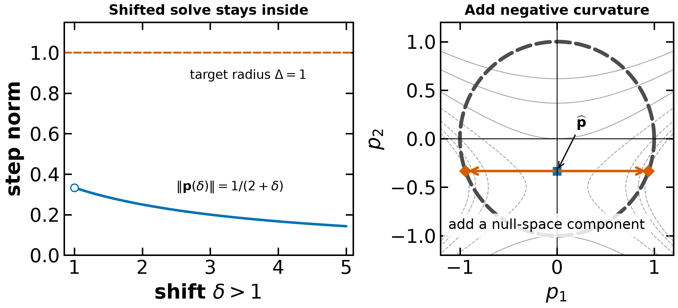
A pure positive-definite correction may suppress this useful curvature. For larger problems, truncated conjugate-gradient trust-region methods detect nonpositive curvature or a boundary crossing and truncate there, avoiding a full eigenvalue decomposition. This is a different mechanism from using an arbitrary indefinite Newton direction in a line search.
Sources: Nocedal and Wright (2006), §4.3, pp. 87--88, Eq. (4.45), and §7.1, pp. 169--175; Biegler (2010), Eqs. (3.54)--(3.55) and Algorithm 3.4, pp. 56--57.