Reference: Sections 3.1 - 3.3 in Biegler (2010)
# Load required Python libraries.
import numpy as np
from scipy import linalg

# Seed the random number generator so this notebook is reproducible
# (Pyomo style guide, section 8).
np.random.seed(0)
Unconstrained Optimization with Approximate Hessian
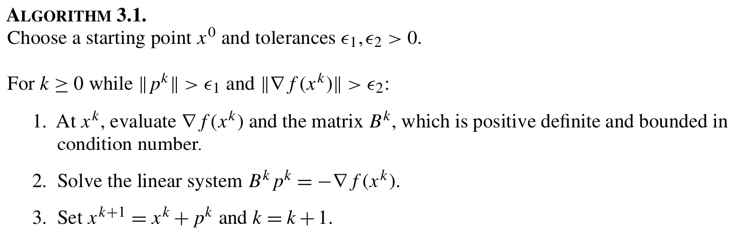
SR1 update is one way to approximate .
Library of helper functions
## Check if any element of array is NaN
def check_nan(A):
    return np.sum(np.isnan(A))


## Calculate gradient with central finite difference
def my_grad_approx(x, f, eps1, verbose=False):
    """
    Calculate gradient of function my_f using central difference formula

    Inputs:
        x - point for which to evaluate gradient
        f - function to consider
        eps1 - perturbation size

    Outputs:
        grad - gradient (vector)
    """

    n = len(x)
    grad = np.zeros(n)

    if verbose:
        print("***** my_grad_approx at x = ", x, "*****")

    for i in range(0, n):

        # Create vector of zeros except eps in position i
        e = np.zeros(n)
        e[i] = eps1

        # Finite difference formula
        my_f_plus = f(x + e)
        my_f_minus = f(x - e)

        # Diagnostics
        if verbose:
            print("e[", i, "] = ", e)
            print("f(x + e[", i, "]) = ", my_f_plus)
            print("f(x - e[", i, "]) = ", my_f_minus)

        grad[i] = (my_f_plus - my_f_minus) / (2 * eps1)

    if verbose:
        print("***** Done. ***** \n")

    return grad


## Calculate Hessian using central finite difference
def my_hes_approx(x, grad, eps2):
    """
    Calculate Hessian of function my_f using central difference formula and my_grad

    Inputs:
        x - point for which to evaluate gradient
        grad - function to calculate the gradient
        eps2 - perturbation size (for Hessian NOT gradient approximation)

    Outputs:
        H - Hessian (matrix)
    """

    n = len(x)
    H = np.zeros([n, n])

    for i in range(0, n):
        # Create vector of zeros except eps in position i
        e = np.zeros(n)
        e[i] = eps2

        # Evaluate gradient twice
        grad_plus = grad(x + e)
        grad_minus = grad(x - e)

        # Notice we are building the Hessian by column (or row)
        H[:, i] = (grad_plus - grad_minus) / (2 * eps2)

    return H


## Linear algebra calculation
def xxT(u):
    """
    Calculates u*u.T to circumvent limitation with SciPy

    Arguments:
    u - numpy 1D array

    Returns:
    u*u.T

    Assume u is a nx1 vector.
    Recall: NumPy does not distinguish between row or column vectors

    u.dot(u) returns a scalar. This function returns an nxn matrix.
    """

    n = len(u)
    A = np.zeros([n, n])
    for i in range(0, n):
        for j in range(0, n):
            A[i, j] = u[i] * u[j]

    return A


## Analyze Hessian
def analyze_hes(B):
    print(B, "\n")

    l = linalg.eigvals(B)
    print("Eigenvalues: ", l, "\n")
Symmetric Rank 1 (SR1) Update
def alg1_sr1(x0, calc_f, calc_grad, eps1, eps2, verbose=False, max_iter=1000):
    """
    Arguments:
        x0 - starting point
        calc_f - function that calculates f(x)
        calc_grad - function that calculates gradient(x)

    Outputs:
        x - iteration history of x (decision variables)
        f - iteration history of f(x) (objective value)
        p - iteration history of p (steps)
        B - Hessian approximation
    """

    # Allocate outputs as empty lists
    x = []
    f = []
    p = []
    grad = []
    B = []

    # Store starting point
    x.append(x0)
    k = 0

    flag = True

    print("Iter. \tf(x) \t\t||grad(x)|| \t||p|| \t\tmin(lambda)")

    while flag and k < max_iter:
        # Evaluate f(x) at current iteration
        f.append(calc_f(x[k]))

        # Evaluate gradient
        grad.append(calc_grad(x[k]))

        if check_nan(grad[k]):
            print("WARNING: gradient calculation returned NaN")
            break

        if verbose:
            print("\n")
            print("k = ", k)
            print("x = ", x[k])
            print("grad = ", grad[k])

        # Update Hessian approximation
        if k == 0:
            # Initialize with identity
            B.append(np.eye(len(x0)))

        else:
            # Change in x
            s = x[k] - x[k - 1]

            # Change in gradient
            y = grad[k] - grad[k - 1]

            # SR1 formulation
            u = y - B[k - 1].dot(s)
            denom = (u).dot(s)

            # Safeguard: skip test for the SR1 update.
            # Only apply the update when
            #     | (y - B^k s)^T s |  >=  C1 * ||s||^2,   C1 > 0
            # and otherwise leave B unchanged. See the "Quasi-Newton Methods"
            # lecture notes, Strategy 1 (SR1), and Biegler (2010), p. 43.
            # If the denominator is (near) zero the rank-one correction is an
            # arbitrarily large, arbitrarily ill-conditioned change built from
            # almost no new information. Note the test is two-sided: it looks at
            # the magnitude only, because -- unlike BFGS -- SR1 is allowed to
            # represent negative curvature.
            C1 = 1e-8

            if abs(denom) >= C1 * s.dot(s):
                # Formula: dB = u * u.T / (u.T * s) if u is a column vector.
                dB = xxT(u) / denom
                skipped = False
            else:
                # Skip the update: B[k] = B[k-1]
                dB = np.zeros((len(x0), len(x0)))
                skipped = True

            if verbose:
                print("s = ", s)
                print("y = ", y)
                print("SR1 update denominator, (y-B[k-1]*s).T*s = ", denom)
                print("SR1 update u = ", u)
                if skipped:
                    print("Skip test |denom| >= C1*||s||^2 failed: update skipped.")
                print("SR1 update u.T*u/(u.T*s) = \n", dB)

            B.append(B[k - 1] + dB)

        if verbose:
            print("B = \n", B[k])

        if check_nan(B[k]):
            print("WARNING: Hessian update returned NaN")
            break

        c = np.linalg.cond(B[k])
        if c > 1e12:
            flag = False
            print("Warning: Hessian approximation is near singular.")
            print("B[k] = \n", B[k])

        else:
            # Calculate step
            p.append(linalg.solve(B[k], -grad[k]))

            if verbose:
                print("p = ", p[k])

            # Take step
            x.append(x[k] + p[k])

            # Calculate norms
            norm_p = linalg.norm(p[k])
            norm_g = linalg.norm(grad[k])

            # Calculate eigenvalues of Hessian (for display only)
            ev = np.real(linalg.eigvals(B[k]))

            # print("k = ",k,"\t"f[k],"\t",norm_g,"\t",norm_p)
            print(
                k,
                "  \t{0: 1.4e} \t{1:1.4e} \t{2:1.4e} \t{3: 1.4e}".format(
                    f[k], norm_g, norm_p, np.min(ev)
                ),
            )

            # Check convergence criteria
            flag = (norm_p > eps1) and (norm_g > eps2)

            # Update iteration counter
            k = k + 1

    print("Done.")
    print("x* = ", x[-1])

    return x, f, p, B


print("Done.")
Done.
def my_f_simple(x):
    return x[0] ** 2 + (x[1] - 1) ** 2


def my_grad_exact(x):
    return np.array([2 * x[0], 2 * (x[1] - 1)])
Near solution
Consider
# Specify convergence criteria
eps1 = 1e-8
eps2 = 1e-4

# Create a Lambda (anonymous) function for gradient calculation
# calc_grad = lambda x : my_grad_approx(x,my_f_simple,1E-6,verbose=False)
calc_grad = lambda x: my_grad_exact(x)

# Specify starting point
x0 = np.array([-0.1, 0.2])

# Call optimization routine
x, f, p, B = alg1_sr1(
    x0, my_f_simple, calc_grad, eps1, eps2, verbose=False, max_iter=50
)

# SR1 Hessian approximation
print("\nSR1 Hessian approximation. B[k] =")
analyze_hes(B[-1])

# Actual Hessian
print("True Hessian at x*. B =")
analyze_hes(my_hes_approx(x[-1], calc_grad, 1e-6))
Iter. f(x) ||grad(x)|| ||p|| min(lambda)
0 6.5000e-01 1.6125e+00 1.6125e+00 1.0000e+00
1 6.5000e-01 1.6125e+00 8.0623e-01 1.0000e+00
2 0.0000e+00 0.0000e+00 0.0000e+00 1.0000e+00
Done.
x* = [0. 1.]
SR1 Hessian approximation. B[k] =
[[1.01538462 0.12307692]
[0.12307692 1.98461538]]
Eigenvalues: [1.+0.j 2.+0.j]
True Hessian at x*. B =
[[2. 0.]
[0. 2.]]
Eigenvalues: [2.+0.j 2.+0.j]
Far from solution
Consider
# Specify starting point
x0 = np.array([-100, 500])

# Call optimization routine
x, f, p, B = alg1_sr1(
    x0, my_f_simple, calc_grad, eps1, eps2, verbose=False, max_iter=50
)

# SR1 Hessian approximation
print("\nSR1 Hessian approximation. B[k] =")
analyze_hes(B[-1])

# Actual Hessian
print("True Hessian at x*. B =")
analyze_hes(my_hes_approx(x[-1], calc_grad, 1e-6))
Iter. f(x) ||grad(x)|| ||p|| min(lambda)
0 2.5900e+05 1.0178e+03 1.0178e+03 1.0000e+00
1 2.5900e+05 1.0178e+03 5.0892e+02 1.0000e+00
2 5.0487e-27 1.4211e-13 1.1604e-13 1.0000e+00
Done.
x* = [-5.1938169e-14 1.0000000e+00]
SR1 Hessian approximation. B[k] =
[[ 1.03860989 -0.19266335]
[-0.19266335 1.96139011]]
Eigenvalues: [1.+0.j 2.+0.j]
True Hessian at x*. B =
[[2. 0.]
[0. 2.]]
Eigenvalues: [2.+0.j 2.+0.j]
Activity/Discussion
Does the number of iterations depend on the starting point for this problem?
How many iterations are needed for Newton’s method to converge for a positive definite quadratic program using exact second derivative information?
Why does the SR1 update not converge to the true Hessian?
Test Case: Example 2.19
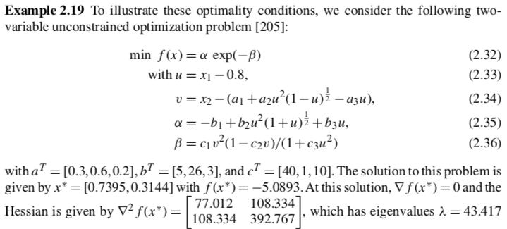
## Define Python function to calculate objective
def my_f_ex_2_19(x, verbose=False):
    """Evaluate function given above at point x

    Inputs:
        x - vector with 2 elements

    Outputs:
        f - function value (scalar)
    """
    # Constants
    a = np.array([0.3, 0.6, 0.2])
    b = np.array([5, 26, 3])
    c = np.array([40, 1, 10])

    # Intermediates. Recall Python indicies start at 0
    u = x[0] - 0.8
    s = np.sqrt(1 - u)
    s2 = np.sqrt(1 + u)
    v = x[1] - (a[0] + a[1] * u**2 * s - a[2] * u)
    alpha = (
        -b[0] + b[1] * u**2 * s2 + b[2] * u
    )  # September 5, 2018: changed 's' to 's2'
    beta = c[0] * v**2 * (1 - c[1] * v) / (1 + c[2] * u**2)
    f = alpha * np.exp(-beta)

    if verbose:
        print("##### my_f at x = ", x, "#####")
        print("u = ", u)
        print("sqrt(1-u) = ", s)
        print("sqrt(1+u) = ", s2)
        print("v = ", v)
        print("alpha = ", alpha)
        print("beta = ", beta)
        print("f(x) = ", f)
        print("##### Done. #####\n")

return f# Create a Lambda (anonymous) function for gradient calculation
calc_grad = lambda x: my_grad_approx(x, my_f_ex_2_19, 1e-6, verbose=False)
# Specify starting point
x0 = np.array([0.3, 0.1])
# Call optimization routine
x, f, p, B = alg1_sr1(
x0, my_f_ex_2_19, calc_grad, eps1, eps2, verbose=False, max_iter=250
)
# SR1 Hessian approximation
print("\nSR1 Hessian approximation. B[k] =")
analyze_hes(B[-1])
# Actual Hessian
print("True Hessian at x*. B =")
analyze_hes(my_hes_approx(x[-1], calc_grad, 1e-6))Iter. f(x) ||grad(x)|| ||p|| min(lambda)
0 -3.6022e-02 8.3847e-01 8.3847e-01 1.0000e+00
1 -4.1276e-02 4.7785e-01 3.0223e-01 1.0000e+00
2 -2.2301e+00 2.1236e+01 3.0865e-01 -6.8856e+01
3 -4.1260e-02 4.4645e-01 1.3053e-01 -6.7478e+01
4 -1.0354e-01 1.1855e+00 1.5062e-01 -7.1805e+01
5 -3.7115e-02 3.9982e-01 1.3096e-02 -5.8783e+01
6 -3.4039e-02 3.6164e-01 5.9865e-02 -1.4365e+01
7 -2.2398e-02 2.0377e-01 4.2988e-02 -9.5209e+00
8 -1.7133e-02 1.1914e-01 4.2522e-02 -6.4394e+00
9 -1.4292e-02 5.7282e-02 2.4810e-02 -4.8015e+00
10 -1.3542e-02 2.5813e-02 1.0353e-02 -2.8612e+00
11 -1.3373e-02 1.0933e-02 8.4091e-03 -1.6117e+00
12 -1.3325e-02 7.7765e-04 7.5906e-04 -1.6030e+00
13 -1.3324e-02 1.7106e-05 1.4129e-05 -1.5761e+00
Done.
x* = [0.80557705 0.96556999]
SR1 Hessian approximation. B[k] =
[[-1.48333926 -0.21589308]
[-0.21589308 -1.07333657]]
Eigenvalues: [-1.57605485+0.j -0.98062098+0.j]
True Hessian at x*. B =
[[-1.47003026 -0.2060227 ]
[-0.2060227 -1.06562155]]
Eigenvalues: [-1.55649865+0.j -0.97915316+0.j]
# Specify starting point
x0 = np.array([-0.1, 0.2])

# Call optimization routine
x, f, p, B = alg1_sr1(
    x0, my_f_ex_2_19, calc_grad, eps1, eps2, verbose=False, max_iter=250
)

# SR1 Hessian approximation
print("\nSR1 Hessian approximation. B[k] =")
analyze_hes(B[-1])

# Actual Hessian
print("True Hessian at x*. B =")
analyze_hes(my_hes_approx(x[-1], calc_grad, 1e-6))
Iter. f(x) ||grad(x)|| ||p|| min(lambda)
0 -4.5540e-04 9.2580e-03 9.2580e-03 1.0000e+00
1 -5.4879e-04 1.0959e-02 5.9578e-02 -1.8395e-01
2 -1.5604e-04 3.4877e-03 2.7627e-02 -1.2568e-01
3 -8.3235e-05 1.9563e-03 3.5000e-02 -5.5390e-02
4 -3.6006e-05 9.0023e-04 2.9559e-02 -3.0011e-02
5 -1.7097e-05 4.4964e-04 2.9246e-02 -1.5078e-02
6 -7.9092e-06 2.1835e-04 2.7389e-02 -7.7836e-03
7 -3.7242e-06 1.0745e-04 2.6349e-02 -3.9664e-03
8 -1.7531e-06 5.2702e-05 2.5208e-02 -2.0268e-03
Done.
x* = [-0.11328951 -0.05033867]
SR1 Hessian approximation. B[k] =
[[ 1.00141633e+00 -4.82365648e-02]
[-4.82365648e-02 2.91945446e-04]]
Eigenvalues: [ 1.00373512+0.j -0.00202684+0.j]
True Hessian at x*. B =
[[ 6.99095467e-05 -2.18304769e-04]
[-2.18304769e-04 -7.02715474e-04]]
Eigenvalues: [ 0.00012732+0.j -0.00076013+0.j]
Activity/Discussion
Classify each candidate solution.
Is the SR1 approximation always positive definite?
Broyden update with Cholesky factorization
As part of Algorithms Homework 3, you will adapt this example and implement the BFGS (Broyden-Fletcher-Goldfarb-Shanno) update formula.
You may decide to use the Cholesky factorization of ,
to make your BFGS update more efficient. (This is not required). Let’s see how to do Cholesky factorization with SciPy.
## Create random P.D. and symmetric matrix
B_ = np.eye(3) + xxT(np.random.normal(0, 1, 3))
print("B = \n", B_, "\n")

## Perform Cholesky factorization.
# By default, lower=False and L is upper triangular. Either works here,
# but we prefer L to be lower triangular for convention.
L = linalg.cholesky(B_, lower=True)
print("L = \n", L, "\n")

## Reconstruct B
print("L*L.T = \n", L.dot(L.T), "\n")
B =
[[4.11188068 0.70589826 1.72654504]
[0.70589826 1.16012579 0.39164906]
[1.72654504 0.39164906 1.95792804]]
L =
[[2.02777728 0. 0. ]
[0.3481143 1.01928515 0. ]
[0.85144708 0.09344604 1.10645097]]
L*L.T =
[[4.11188068 0.70589826 1.72654504]
[0.70589826 1.16012579 0.39164906]
[1.72654504 0.39164906 1.95792804]]