Reference: Section 2.4.2 in Biegler (2010)
import sys

if "google.colab" in sys.modules:
    !wget "https://raw.githubusercontent.com/ndcbe/optimization/main/notebooks/helper.py"
    # We do not need to install Pyomo or Ipopt, but we do want to format our plots
    # helper.easy_install()
    import helper
else:
    sys.path.insert(0, "../")
    import helper
helper.set_plotting_style()

# Load required Python libraries.
import matplotlib.pyplot as plt
import numpy as np
from scipy import linalg
Newton models for equations and optimization¶
A row-oriented Jacobian for equations¶
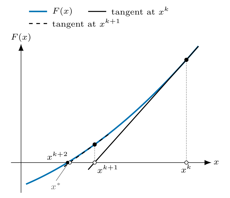
Let be open and differentiable. Define for . Linearizing at fixed gives
with the quadratic remainder when the Jacobian is locally Lipschitz. Newton sets the linear model to zero and solves
The actual residual at the update need not be zero. The row-oriented Jacobian requires no extra transpose. An inverse is useful in analysis, but a numerical implementation solves the linear system.
A quadratic model for a scalar objective¶
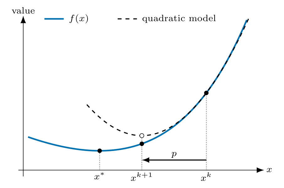
For on an open , write and . With fixed,
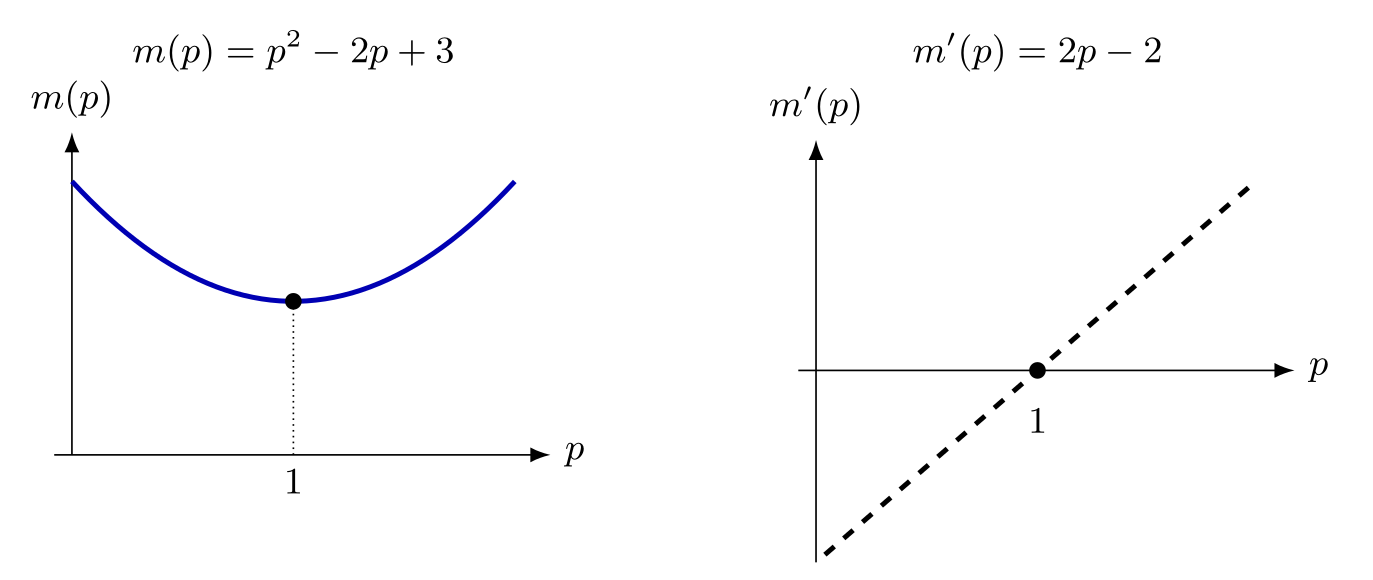
Differentiating the model with respect to the chosen displacement gives
This computes a model stationary point. It is the model minimum if . The model equals a quadratic objective exactly; for a nonlinear objective with locally Lipschitz Hessian its value remainder is .
Sources: Biegler (2010), Eqs. (2.37)–(2.39), pp. 34–35; Nocedal and Wright (2006), §11.1, pp. 274–277. The gradient in the numerical examples below is a column vector.
Curvature, descent, and step length¶
A strict local minimum need not have a positive-definite Hessian: at zero is a counterexample. The sufficient second-order conditions explicitly require a zero gradient and positive-definite Hessian. Continuity then preserves positive definiteness in a small neighborhood.
For , a direction is descent when . If and , then
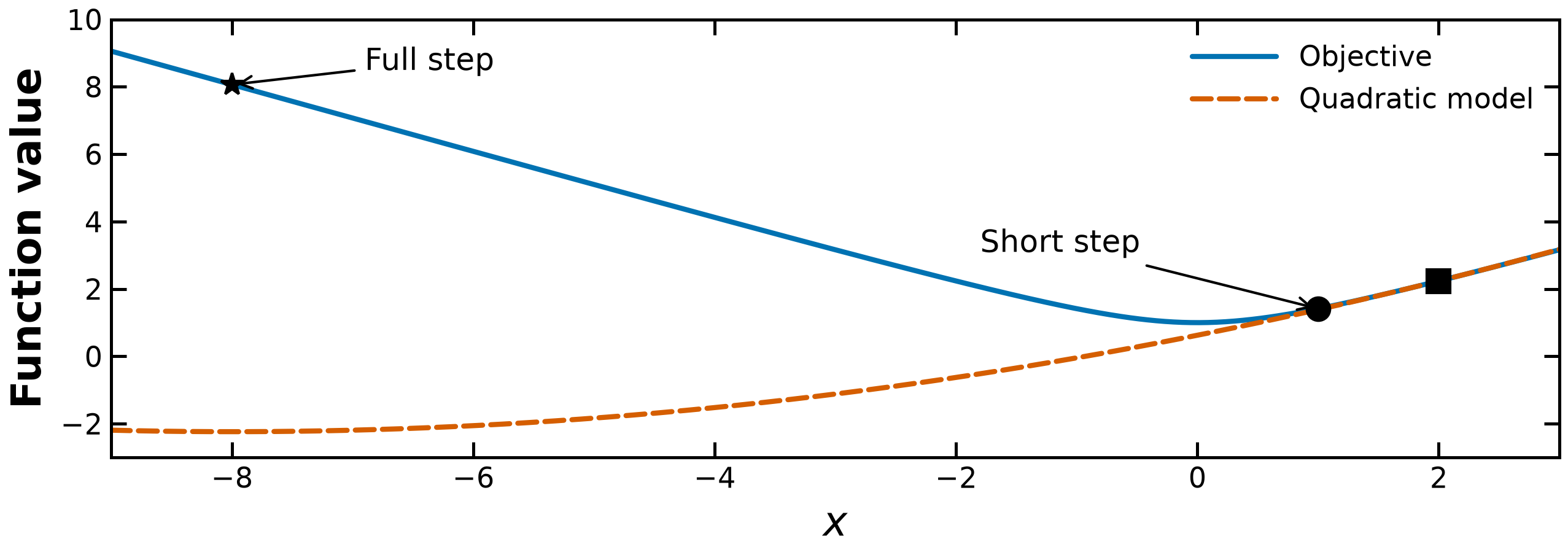
This guarantees decrease for sufficiently small positive step lengths. It does not guarantee decrease for every . For a objective, the exact Taylor identity is
At fixed , the negative term dominates the bounded remainder for small . The intermediate point includes .
A singular Hessian does not specify a unique basic Newton step. An indefinite Hessian can produce an ascent direction; an inaccurate positive-definite model can still overshoot. These are distinct reasons to modify curvature or control the accepted step length.
Sources: Biegler (2010), Eq. (2.40), p. 34, and §3.1, pp. 39–40; Nocedal and Wright (2006), pp. 22 and 46–47.
Algorithm 2.1: basic unit-step Newton¶
The following reference version adapts Biegler’s Algorithm 2.1 so each quantity is evaluated before it is tested.
Choose , gradient tolerance , and step tolerance .
Evaluate and . A small gradient reports an approximately stationary candidate.
If the Hessian is singular, report failure of the basic solve; otherwise solve .
A small step reports limited numerical movement, together with the current gradient norm.
Otherwise take and repeat.
A candidate must still be classified; neither a small step nor an approximate Hessian proves a minimum. The diagnostic implementation below retains a post-step convergence test and also checks NaN derivatives, severe conditioning, and an iteration limit. Its experiments deliberately include failure cases.
Source: Biegler (2010), Algorithm 2.1, p. 35.
Helper Function¶
## Calculate gradient with central finite difference
def my_grad_approx(x, f, eps1, verbose=False):
    """
    Calculate gradient of function my_f using central difference formula

    Inputs:
        x - point for which to evaluate gradient
        f - function to consider
        eps1 - perturbation size

    Outputs:
        grad - gradient (vector)
    """

    n = len(x)
    grad = np.zeros(n)

    if verbose:
        print("***** my_grad_approx at x = ", x, "*****")

    for i in range(0, n):

        # Create vector of zeros except eps in position i
        e = np.zeros(n)
        e[i] = eps1

        # Finite difference formula
        my_f_plus = f(x + e)
        my_f_minus = f(x - e)

        # Diagnostics
        if verbose:
            print("e[", i, "] = ", e)
            print("f(x + e[", i, "]) = ", my_f_plus)
            print("f(x - e[", i, "]) = ", my_f_minus)

        grad[i] = (my_f_plus - my_f_minus) / (2 * eps1)

    if verbose:
        print("***** Done. ***** \n")

    return grad


## Calculate gradient using central finite difference and my_hes_approx
def my_hes_approx(x, grad, eps2):
    """
    Calculate Hessian of function my_f using central difference formula and my_grad

    Inputs:
        x - point for which to evaluate gradient
        grad - function to calculate the gradient
        eps2 - perturbation size (for Hessian NOT gradient approximation)

    Outputs:
        H - Hessian (matrix)
    """

    n = len(x)
    H = np.zeros([n, n])

    for i in range(0, n):
        # Create vector of zeros except eps in position i
        e = np.zeros(n)
        e[i] = eps2

        # Evaluate gradient twice
        grad_plus = grad(x + e)
        grad_minus = grad(x - e)

        # Notice we are building the Hessian by column (or row)
        H[:, i] = (grad_plus - grad_minus) / (2 * eps2)

    return H


def check_nan(A):
    return np.sum(np.isnan(A))


## Analyze Hessian.
def analyze_hes(B):
    print(B, "\n")

    if not check_nan(B):
        # Calculate eigenvalues
        l = linalg.eigvals(B)
        print("Eigenvalues: ", l, "\n")
Algorithm 1 Python Implementation¶
## Implement Alg 1 in a function
def alg1(x0, calc_f, calc_grad, calc_hes, eps1, eps2, verbose=False, max_iter=250):
    """
    Arguments:
        x0 - starting point
        calc_f - function that calculates f(x)
        calc_grad - function that calculates gradient(x)
        calc_hes - function that calculates hessian(x)

    Outputs:
        x - iteration history of x (decision variables)
        f - iteration history of f(x) (objective value)
        p - iteration history of p (steps)
    """

    # Allocate outputs as empty lists
    x = []
    f = []
    p = []

    # Store starting point
    x.append(x0)
    k = 0

    flag = True

    print("Iter. \tf(x) \t\t||grad(x)|| \t||p|| \t\tmin(lambda)")

    while flag:
        # Evaluate f(x) at current iteration
        f.append(calc_f(x[k]))

        # Evaluate gradient
        grad = calc_grad(x[k])

        if check_nan(grad):
            print("WARNING: gradient calculation returned NaN")
            break

        # Evaluate Hessian
        hes = calc_hes(x[k])

        if check_nan(hes):
            print("WARNING: Hessian calculation returned NaN")
            break

        if verbose:
            print("\n")
            print("k = ", k)
            print("x = ", x[k])
            print("grad = ", grad)
            print("hes = \n", hes)

        # Check if singular via condition number
        c = np.linalg.cond(hes)
        if c > 1e12:
            flag = False
            print("Warning: Hessian is near singular.")

        else:
            # Calculate step

            p.append(linalg.solve(hes, -grad))

            if verbose:
                print("p = ", p[k])

            # Take step. x[k+1] = x[k] + p[k]
            x.append(x[k] + p[k])

            # Calculate norms
            norm_p = linalg.norm(p[k])
            norm_g = linalg.norm(grad)

            # Calculate eigenvalues (for display only)
            ev = np.real(linalg.eigvals(hes))

            # print("k = ",k,"\t"f[k],"\t",norm_g,"\t",norm_p)
            print(
                k,
                "  \t{0: 1.4e} \t{1:1.4e} \t{2:1.4e} \t{3: 1.4e}".format(
                    f[k], norm_g, norm_p, np.min(ev)
                ),
            )

            # Check convergence criteria
            flag = (norm_p > eps1) and (norm_g > eps2)

            # Update iteration counter
            k = k + 1

        if k > max_iter:
            flag = False
            print("Maximum number of iterations.")
    print("Done.")
    print("x* = ", x[-1])

    return x, f, p
Quantified rates of convergence¶
Let and . The convergence is at least Q-linear when
It is at least Q-quadratic when
These are eventual upper bounds; a sequence can satisfy a stronger rate too. For , gives , while gives . Strict minimality by itself supplies neither the rate nor the theorem’s nondegeneracy: unit-step Newton on has for , so its exact error ratio is , and .
Source: Nocedal and Wright (2006), Appendix A.2, Eq. (A.34), p. 619. The following theorem and proofs specify the neighborhood and constants required for Newton’s quadratic bounds.
Quadratic Convergence Proof¶
Theorem 2.20 (Biegler, 2010)
Assume on an open neighborhood of , with Lipschitz Hessian there, , and . Then, by applying Algorithm 2.1 and with a sufficiently close , there exists a constant such that:
The convergence rate for is quadratic, i.e.,
The convergence rate for is also quadratic
Iterate-error proof and the integral-norm tools¶
Use the Euclidean vector norm and its induced matrix norm. The bounds needed here are
Consequently,
This uses induced-norm submultiplicativity and the triangle inequality for an integral, not a scalar Cauchy–Schwarz inequality.
For the exact gradient identity, define . The chain rule gives . Applying the one-variable fundamental theorem of calculus to each component and integrating from zero to one yields
In one dimension, substitution , turns the right side into , including negative through the oriented integral.
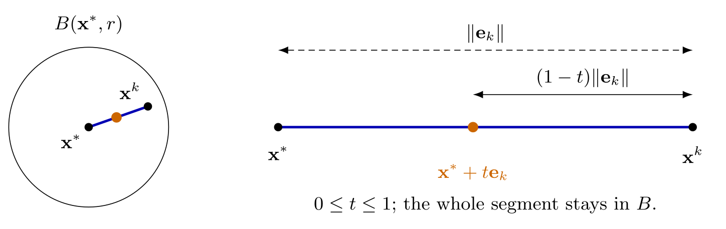
Now set and . In a small convex ball around the nondegenerate stationary point, continuity bounds ; let be a Hessian Lipschitz constant. Subtracting the zero gradient at gives
The distance from the intermediate point to is , so
Choose the initial ball radius small enough that . The estimate then decreases the error and keeps every subsequent iterate in the ball, closing the local induction. Using the looser constant is also valid, but integrating the distance explicitly gives .
Sources: Biegler (2010), Theorem 2.14, pp. 27–28, and Theorem 2.20, p. 35, with the corrected segment in the errata. The prepared error-segment sketch in the lecture represents the same identity.
Gradient-residual proof¶
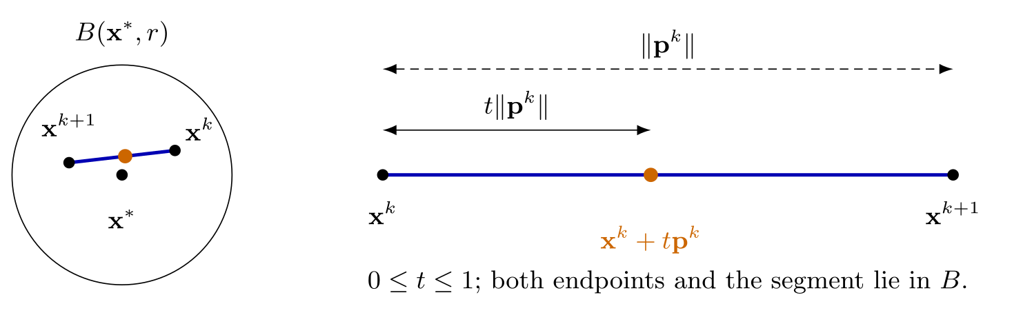
The iterate-error proof keeps both endpoints of each Newton step in the same convex ball. Its segment stays there, so the Hessian Lipschitz and inverse bounds apply. Since ,
The intermediate point is from . Thus
The last inequality uses . Small steps alone do not imply this rate: the nonsingular limiting Hessian and Lipschitz hypotheses do the work.
Source: Biegler (2010), Theorem 2.20 and Eq. (2.43), p. 35.
Test Problem¶
Example 2.19 Consider the following two-variable unconstrained optimization problem:
with
The book reports the rounded candidate with .
The nearby exact stationary point has zero gradient; rounding its coordinates does not preserve exact stationarity. The book reports the following approximate Hessian there:
which has eigenvalues and .
Source: Biegler (2010), Example 2.19, p. 30. The canonical optimality notebook compares rounded and refined points and reports actual derivative residuals; the Newton experiments below use the same objective for a distinct iteration task.
## Define Python function to calculate objective
def my_f(x, verbose=False):
    """Evaluate function given above at point x

    Inputs:
        x - vector with 2 elements

    Outputs:
        f - function value (scalar)
    """
    # Constants
    a = np.array([0.3, 0.6, 0.2])
    b = np.array([5, 26, 3])
    c = np.array([40, 1, 10])

    # Intermediates. Recall Python indices start at 0
    u = x[0] - 0.8
    s = np.sqrt(1 - u)
    s2 = np.sqrt(1 + u)
    v = x[1] - (a[0] + a[1] * u**2 * s - a[2] * u)
    alpha = (
        -b[0] + b[1] * u**2 * s2 + b[2] * u
    )  # September 5, 2018: changed 's' to 's2'
    beta = c[0] * v**2 * (1 - c[1] * v) / (1 + c[2] * u**2)
    f = alpha * np.exp(-beta)

    if verbose:
        print("##### my_f at x = ", x, "#####")
        print("u = ", u)
        print("sqrt(1-u) = ", s)
        print("sqrt(1+u) = ", s2)
        print("v = ", v)
        print("alpha = ", alpha)
        print("beta = ", beta)
        print("f(x) = ", f)
        print("##### Done. #####\n")

    return f
Starting Point Near Optimal Solution¶
## Test on example

# Specify convergence criteria
eps1 = 1e-8
eps2 = 1e-4

# Create a Lambda (anonymous) function for gradient calculation
calc_grad = lambda x: my_grad_approx(x, my_f, 1e-6)

# Create a Lambda (anonymous) function for Hessian calculation
calc_hes = lambda x: my_hes_approx(x, calc_grad, 1e-6)

# Specify starting point
x0 = np.array([0.7, 0.3])

# Call optimization routine
x, f, p = alg1(x0, my_f, calc_grad, calc_hes, eps1, eps2)

# Actual Hessian
print("Hessian at x*= ")
analyze_hes(my_hes_approx(x[-1], calc_grad, 1e-6))
Iter. f(x) ||grad(x)|| ||p|| min(lambda)
0 -4.9246e+00 1.0874e+01 4.1946e-02 4.9368e+01
1 -5.0888e+00 6.2736e-01 1.9752e-03 4.2541e+01
2 -5.0893e+00 2.4210e-03 3.0032e-05 4.3424e+01
3 -5.0893e+00 2.9199e-07 3.1620e-09 4.3418e+01
Done.
x* = [0.73950546 0.3143601 ]
Hessian at x*=
[[ 77.01173033 108.33423048]
[108.33423048 392.76693009]]
Eigenvalues: [ 43.41702924+0.j 426.36163117+0.j]
Activity: A Different Starting Point¶
Try with
# Specify starting point
x0 = np.array([0, 0])

# Call optimization routine
x, f, p = alg1(x0, my_f, calc_grad, calc_hes, eps1, eps2)

# Actual Hessian
print("Hessian at x* = ")
analyze_hes(my_hes_approx(x[-1], calc_grad, 1e-6))
Iter. f(x) ||grad(x)|| ||p|| min(lambda)
0 1.6212e-06 1.5568e-04 3.8590e-02 -2.9496e-03
1 5.4102e-07 5.5405e-05 3.6202e-02 -1.0900e-03
Done.
x* = [-0.00124597 -0.07478209]
Hessian at x* =
[[0.0001531 0.00055527]
[0.00055527 0.00014766]]
Eigenvalues: [ 0.00070565+0.j -0.00040489+0.j]
Activity: Let’s break it¶
Activity: Try . Why does the gradient or Hessian return NaN? Hint: redefine calc_grad and create my_f_verbose using verbose=True.
# Specify starting point
x0 = np.array([-0.2, -0.2])

# Create a Lambda (anonymous) function for f(x) calculation with verbose output
my_f_verbose = lambda x: my_f(x, verbose=True)

# Create a Lambda (anonymous) function for gradient calculation
calc_grad = lambda x: my_grad_approx(x, my_f_verbose, 1e-6, verbose=True)

# Call optimization routine
x, f, p = alg1(x0, my_f, calc_grad, calc_hes, eps1, eps2, verbose=True)

# Actual Hessian
print("Hessian at x* = ")
analyze_hes(my_hes_approx(x[-1], calc_grad, 1e-6))
Iter. f(x) ||grad(x)|| ||p|| min(lambda)
***** my_grad_approx at x = [-0.2 -0.2] *****
##### my_f at x = [-0.199999 -0.2 ] #####
u = -0.9999990000000001
sqrt(1-u) = 1.4142132088196604
sqrt(1+u) = 0.0009999999999588667
v = -1.5485260282367943
alpha = -7.973997052001044
beta = 22.222565160998283
f(x) = -1.780486346234917e-09
##### Done. #####
##### my_f at x = [-0.200001 -0.2 ] #####
u = -1.0000010000000001
sqrt(1-u) = 1.4142139159264415
sqrt(1+u) = nan
v = -1.5485302466134128
alpha = nan
beta = 22.222642208927322
f(x) = nan
##### Done. #####
e[ 0 ] = [1.e-06 0.e+00]
f(x + e[ 0 ]) = -1.780486346234917e-09
f(x - e[ 0 ]) = nan
##### my_f at x = [-0.2 -0.199999] #####
u = -1.0
sqrt(1-u) = 1.4142135623730951
sqrt(1+u) = 0.0
v = -1.548527137423857
alpha = -8.0
beta = 22.222566263573963
f(x) = -1.786290485440547e-09
##### Done. #####
##### my_f at x = [-0.2 -0.200001] #####
u = -1.0
sqrt(1-u) = 1.4142135623730951
sqrt(1+u) = 0.0
v = -1.548529137423857
alpha = -8.0
beta = 22.22264110629725
f(x) = -1.7861567995988046e-09
##### Done. #####
e[ 1 ] = [0.e+00 1.e-06]
f(x + e[ 1 ]) = -1.786290485440547e-09
f(x - e[ 1 ]) = -1.7861567995988046e-09
***** Done. *****
WARNING: gradient calculation returned NaN
Done.
x* = [-0.2 -0.2]
Hessian at x* =
***** my_grad_approx at x = [-0.199999 -0.2 ] *****
##### my_f at x = [-0.199998 -0.2 ] #####
u = -0.999998
sqrt(1-u) = 1.414212855266137
sqrt(1+u) = 0.0014142135623541761
v = -1.5485239190522238
alpha = -7.963224594456855
beta = 22.22252663717692
f(x) = -1.778149501075135e-09
##### Done. #####
##### my_f at x = [-0.2 -0.2] #####
u = -1.0
sqrt(1-u) = 1.4142135623730951
sqrt(1+u) = 0.0
v = -1.5485281374238569
alpha = -8.0
beta = 22.22260368491507
f(x) = -1.7862236413056787e-09
##### Done. #####
e[ 0 ] = [1.e-06 0.e+00]
f(x + e[ 0 ]) = -1.778149501075135e-09
f(x - e[ 0 ]) = -1.7862236413056787e-09
##### my_f at x = [-0.199999 -0.199999] #####
u = -0.9999990000000001
sqrt(1-u) = 1.4142132088196604
sqrt(1+u) = 0.0009999999999588667
v = -1.5485250282367944
alpha = -7.973997052001044
beta = 22.222527739675733
f(x) = -1.7805529756354463e-09
##### Done. #####
##### my_f at x = [-0.199999 -0.200001] #####
u = -0.9999990000000001
sqrt(1-u) = 1.4142132088196604
sqrt(1+u) = 0.0009999999999588667
v = -1.5485270282367944
alpha = -7.973997052001044
beta = 22.222602582361898
f(x) = -1.7804197192545872e-09
##### Done. #####
e[ 1 ] = [0.e+00 1.e-06]
f(x + e[ 1 ]) = -1.7805529756354463e-09
f(x - e[ 1 ]) = -1.7804197192545872e-09
***** Done. *****
***** my_grad_approx at x = [-0.200001 -0.2 ] *****
##### my_f at x = [-0.2 -0.2] #####
u = -1.0
sqrt(1-u) = 1.4142135623730951
sqrt(1+u) = 0.0
v = -1.5485281374238569
alpha = -8.0
beta = 22.22260368491507
f(x) = -1.7862236413056787e-09
##### Done. #####
##### my_f at x = [-0.200002 -0.2 ] #####
u = -1.000002
sqrt(1-u) = 1.4142142694796995
sqrt(1+u) = nan
v = -1.5485323558054604
alpha = nan
beta = 22.222680733035
f(x) = nan
##### Done. #####
e[ 0 ] = [1.e-06 0.e+00]
f(x + e[ 0 ]) = -1.7862236413056787e-09
f(x - e[ 0 ]) = nan
##### my_f at x = [-0.200001 -0.199999] #####
u = -1.0000010000000001
sqrt(1-u) = 1.4142139159264415
sqrt(1+u) = nan
v = -1.5485292466134128
alpha = nan
beta = 22.22260478756765
f(x) = nan
##### Done. #####
##### my_f at x = [-0.200001 -0.200001] #####
u = -1.0000010000000001
sqrt(1-u) = 1.4142139159264415
sqrt(1+u) = nan
v = -1.548531246613413
alpha = nan
beta = 22.222679630328063
f(x) = nan
##### Done. #####
e[ 1 ] = [0.e+00 1.e-06]
f(x + e[ 1 ]) = nan
f(x - e[ 1 ]) = nan
***** Done. *****
***** my_grad_approx at x = [-0.2 -0.199999] *****
##### my_f at x = [-0.199999 -0.199999] #####
u = -0.9999990000000001
sqrt(1-u) = 1.4142132088196604
sqrt(1+u) = 0.0009999999999588667
v = -1.5485250282367944
alpha = -7.973997052001044
beta = 22.222527739675733
f(x) = -1.7805529756354463e-09
##### Done. #####
##### my_f at x = [-0.200001 -0.199999] #####
u = -1.0000010000000001
sqrt(1-u) = 1.4142139159264415
sqrt(1+u) = nan
v = -1.5485292466134128
alpha = nan
beta = 22.22260478756765
f(x) = nan
##### Done. #####
e[ 0 ] = [1.e-06 0.e+00]
f(x + e[ 0 ]) = -1.7805529756354463e-09
f(x - e[ 0 ]) = nan
##### my_f at x = [-0.2 -0.199998] #####
u = -1.0
sqrt(1-u) = 1.4142135623730951
sqrt(1+u) = 0.0
v = -1.548526137423857
alpha = -8.0
beta = 22.222528842273906
f(x) = -1.7863573320035263e-09
##### Done. #####
##### my_f at x = [-0.2 -0.2] #####
u = -1.0
sqrt(1-u) = 1.4142135623730951
sqrt(1+u) = 0.0
v = -1.5485281374238569
alpha = -8.0
beta = 22.22260368491507
f(x) = -1.7862236413056787e-09
##### Done. #####
e[ 1 ] = [0.e+00 1.e-06]
f(x + e[ 1 ]) = -1.7863573320035263e-09
f(x - e[ 1 ]) = -1.7862236413056787e-09
***** Done. *****
***** my_grad_approx at x = [-0.2 -0.200001] *****
##### my_f at x = [-0.199999 -0.200001] #####
u = -0.9999990000000001
sqrt(1-u) = 1.4142132088196604
sqrt(1+u) = 0.0009999999999588667
v = -1.5485270282367944
alpha = -7.973997052001044
beta = 22.222602582361898
f(x) = -1.7804197192545872e-09
##### Done. #####
##### my_f at x = [-0.200001 -0.200001] #####
u = -1.0000010000000001
sqrt(1-u) = 1.4142139159264415
sqrt(1+u) = nan
v = -1.548531246613413
alpha = nan
beta = 22.222679630328063
f(x) = nan
##### Done. #####
e[ 0 ] = [1.e-06 0.e+00]
f(x + e[ 0 ]) = -1.7804197192545872e-09
f(x - e[ 0 ]) = nan
##### my_f at x = [-0.2 -0.2] #####
u = -1.0
sqrt(1-u) = 1.4142135623730951
sqrt(1+u) = 0.0
v = -1.5485281374238569
alpha = -8.0
beta = 22.22260368491507
f(x) = -1.7862236413056787e-09
##### Done. #####
##### my_f at x = [-0.2 -0.200002] #####
u = -1.0
sqrt(1-u) = 1.4142135623730951
sqrt(1+u) = 0.0
v = -1.548530137423857
alpha = -8.0
beta = 22.222678527720475
f(x) = -1.7860899603198772e-09
##### Done. #####
e[ 1 ] = [0.e+00 1.e-06]
f(x + e[ 1 ]) = -1.7862236413056787e-09
f(x - e[ 1 ]) = -1.7860899603198772e-09
***** Done. *****
[[ nan nan]
[ nan -2.42801152e-06]]
/var/folders/b1/m1_w6rrd109bgym0_8fsxw_80000gp/T/ipykernel_92029/2873126429.py:19: RuntimeWarning: invalid value encountered in sqrt
  s2 = np.sqrt(1 + u)
Activity: Use in place of Hessian¶
Use the displayed constant model in place of the Hessian. This computes a gradient step with scale ; it does not compute the objective’s actual curvature.
def eye_hes(x):
    return 50 * np.eye(len(x))
Test with starting point
# Specify starting point
x0 = np.array([0.7, 0.3])

# Create a Lambda (anonymous) function for gradient calculation
calc_grad = lambda x: my_grad_approx(x, my_f, 1e-6, verbose=False)

# Call optimization routine
x, f, p = alg1(x0, my_f, calc_grad, eye_hes, eps1, eps2, max_iter=25, verbose=False)

# Actual Hessian
print("Hessian at x* = ")
analyze_hes(my_hes_approx(x[-1], calc_grad, 1e-6))
Iter. f(x) ||grad(x)|| ||p|| min(lambda)
0 -4.9246e+00 1.0874e+01 2.1749e-01 5.0000e+01
1 -1.4795e+00 1.6883e+01 3.3765e-01 5.0000e+01
2 -1.8403e+00 2.6363e+01 5.2725e-01 5.0000e+01
3 -1.2461e-01 1.6246e+00 3.2493e-02 5.0000e+01
4 -1.9169e-01 2.5753e+00 5.1507e-02 5.0000e+01
5 -3.8498e-01 5.2112e+00 1.0422e-01 5.0000e+01
6 -1.4594e+00 1.6836e+01 3.3673e-01 5.0000e+01
7 -1.9249e+00 2.6467e+01 5.2934e-01 5.0000e+01
8 -1.1531e-01 1.5097e+00 3.0195e-02 5.0000e+01
9 -1.7247e-01 2.3351e+00 4.6703e-02 5.0000e+01
10 -3.2703e-01 4.5030e+00 9.0059e-02 5.0000e+01
11 -1.0837e+00 1.3485e+01 2.6971e-01 5.0000e+01
12 -4.4497e+00 2.0946e+01 4.1891e-01 5.0000e+01
13 -1.6236e-01 2.1013e+00 4.2026e-02 5.0000e+01
14 -2.8114e-01 3.6906e+00 7.3812e-02 5.0000e+01
15 -7.2912e-01 9.1154e+00 1.8231e-01 5.0000e+01
16 -4.1506e+00 2.1547e+01 4.3094e-01 5.0000e+01
17 -5.4382e-03 2.2424e-01 4.4848e-03 5.0000e+01
18 -6.5332e-03 2.6508e-01 5.3017e-03 5.0000e+01
19 -8.0846e-03 3.2179e-01 6.4357e-03 5.0000e+01
20 -1.0414e-02 4.0482e-01 8.0965e-03 5.0000e+01
21 -1.4199e-02 5.3561e-01 1.0712e-02 5.0000e+01
22 -2.1098e-02 7.6415e-01 1.5283e-02 5.0000e+01
23 -3.6112e-02 1.2322e+00 2.4644e-02 5.0000e+01
24 -8.0386e-02 2.4796e+00 4.9592e-02 5.0000e+01
25 -3.1729e-01 7.8096e+00 1.5619e-01 5.0000e+01
Maximum number of iterations.
Done.
x* = [0.71010106 0.23551614]
Hessian at x* =
[[ 45.2508031 7.93765054]
[ 7.93765054 147.99461656]]
Eigenvalues: [ 44.64118334+0.j 148.60423633+0.j]
Test with starting point
# Specify starting point
x0 = np.array([0.0, 0.0])

# Call optimization routine
x, f, p = alg1(x0, my_f, calc_grad, calc_hes, eps1, eps2)

# Actual Hessian
print("Hessian at x*= ")
analyze_hes(my_hes_approx(x[-1], calc_grad, 1e-6))
Iter. f(x) ||grad(x)|| ||p|| min(lambda)
0 1.6212e-06 1.5568e-04 3.8590e-02 -2.9496e-03
1 5.4102e-07 5.5405e-05 3.6202e-02 -1.0900e-03
Done.
x* = [-0.00124597 -0.07478209]
Hessian at x*=
[[0.0001531 0.00055527]
[0.00055527 0.00014766]]
Eigenvalues: [ 0.00070565+0.j -0.00040489+0.j]
Adjust Hessian with Levenberg-Marquardt Correction¶
def adjusted_hes(x, grad, eps2, eps3, verbose=False):

    # Estimate Hessian with finite difference
    hes = my_hes_approx(x, grad, eps2)

    # Calculate eigenvalues
    l, V = linalg.eig(hes)
    smallest_ev = np.min(np.real(l))

    # Calculate modification
    delta = 0
    if smallest_ev - eps3 < 0:
        delta = -smallest_ev + eps3

    if verbose:
        print("Added ({0:1.4e})*I in LM correction.".format(delta))

    # Adjust hessian with Levenberg-Marquardt Correction
    return V.dot(np.diag(np.real(l)) + delta * np.eye(len(x))).dot(V.T)
# Specify starting point
x0 = np.array([-0.1, -0.1])
# Create a Lambda (anonymous) function for Hessian calculation
calc_hes = lambda x: adjusted_hes(x, calc_grad, 1e-6, 1e-3, verbose=True)
# Call optimization routine
x, f, p = alg1(x0, my_f, calc_grad, calc_hes, eps1, eps2, verbose=False)
# Actual Hessian
print("Hessian at x*= ")
analyze_hes(my_hes_approx(x[-1], calc_grad, 1e-6))Iter. f(x) ||grad(x)|| ||p|| min(lambda)
Added (1.2030e-03)*I in LM correction.
0 -2.0284e-07 6.5946e-06 6.5923e-03 1.0000e-03
Done.
x* = [-0.09849776 -0.0935812 ]
Hessian at x*=
[[ 4.20491243e-05 -5.31304857e-05]
[-5.31304857e-05 -2.35437850e-04]]
Eigenvalues: [ 5.18741524e-05+0.j -2.45262878e-04+0.j]
Enhancement Ideas¶
Here are some ideas to improve this notebook:
Plot the test function
On the plot of the test function, visualize the solution path