import matplotlib.pyplot as plt
import numpy as np
Define Test Function and Derivatives
Let’s get started by defining a test function we will use throughout the notebook.
Consider a scalar function to allow for easier visualization. Let
## Define f(x)
f = lambda x: 0.5 * (x - 1) ** 4 + (x + 1) ** 3 - 10 * x**2 + 5 * x

## Define f'(x)
df = lambda x: 6 - 8 * x - 3 * x**2 + 2 * x**3

## Define f''(x)
ddf = lambda x: -8 - 6 * x + 6 * x**2
plt.figure()
xplt = np.arange(-3, 4, 0.1)
fplt = f(xplt)
dfplt = df(xplt)
ddfplt = ddf(xplt)
# House cycle in order (figures/dowling.mplstyle): black solid, blue dashed,
# orange dash-dot. These were matplotlib's "b"/"r"/"g", which are outside the
# Okabe-Ito palette the rest of the notebook now uses.
plt.plot(xplt, fplt, label="f(x)", color="black", linestyle="-")
plt.plot(xplt, dfplt, label="f'(x)", color="#0072B2", linestyle="--")
plt.plot(xplt, ddfplt, label="f''(x)", color="#E69F00", linestyle="-.")
plt.xlabel("x")
plt.legend()
plt.grid()
plt.show()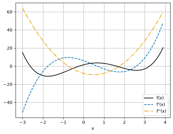
Geometric Insights into Newton Steps
Motivation
We can interpret Newton-type methods for unconstrained optimization as root finding of .
At iteration , we assemble an approximation to using a Taylor series expansion:
and solve for such that . This gives:
The choice of determines the algorithm classification:
Pure Newton Method,
Steepest Descent, , where scalar is sometimes known as the dampening factor
Levenberg-Marquardt, , where scalar is chosen to ensure is positive definite.
Broyden Methods, is approximated using history of gradient evaluations, i.e., . We will study the SR1 and BFGS formulas in this family of methods.
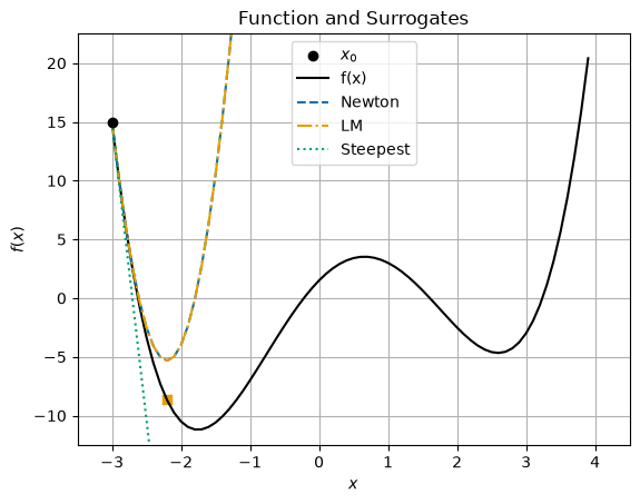
This section explores how choosing impacts the shape of the approximation and calculated step.
Compute and Plot Steps
Define a function that:
Computes the i. Newton, ii. Levenberg-Marquardt and iii. Steepest Descent Step for a given starting point
Plots the step in terms of and
def calc_step(x0, epsLM):

    # Evaluate f(x0), f'(x0) and f''(x0)
    f0 = f(x0)
    df0 = df(x0)
    ddf0 = ddf(x0)
    print("x0 = ", x0)
    print("f(x0) =", f0)
    print("f'(x0) =", df0)
    print("f''(x0) =", ddf0)

    ### Calculate steps

    # Newton Step
    xN = x0 - df0 / ddf0

    print("\n### Newton Step ###")
    print("xN = ", xN)
    print("pN = xN - x0 = ", xN - x0)
    f_xN = f(xN)
    print("f(xN) = ", f_xN)
    print("f(xN) - f(x0) = ", f_xN - f0)

    # Levenberg-Marquardt Step
    # Recall the eigenvalue of a 1x1 matrix is just that value
    dffLM = np.amax([ddf0, epsLM])
    xLM = x0 - df0 / dffLM

    print("\n### Levenberg-Marquardt Step ###")
    print("xLM = ", xLM)
    print("pLM = xLM - x0 = ", xLM - x0)
    f_xLM = f(xLM)
    print("f(xLM) = ", f_xLM)
    print("f(xLM) - f(x0) = ", f_xLM - f0)

    # Steepest Descent Step
    xSD = x0 - df0 / 1

    print("\n### Steepest Descent Step ###")
    print("xSD = ", xSD)
    print("pSD = xSD - x0 = ", xSD - x0)
    f_xSD = f(xSD)
    print("f(xSD) = ", f_xSD)
    print("f(xSD) - f(x0) = ", f_xSD - f0)

    ### Plot Surrogates on x vs f(x)

    ### Plot f(x)
    # Okabe-Ito colours paired with distinct linestyles and markers, in the
    # order used by figures/dowling.mplstyle: black solid, blue dashed, orange
    # dash-dot, bluish green dotted. All three surrogates used to be dashed and
    # were told apart by colour alone, which does not survive a photocopy.
    plt.figure()
    plt.scatter(x0, f0, label="$x_0$", color="black", zorder=5)
    plt.plot(xplt, fplt, label="f(x)", color="black", linestyle="-")

    ### Plot approximation for Newton's method
    fN = lambda x: f0 + df0 * (x - x0) + 0.5 * ddf0 * (x - x0) ** 2
    plt.plot(xplt, fN(xplt), label="Newton", linestyle="--", color="#0072B2")
    plt.scatter(xN, f(xN), color="#0072B2", marker="x")

    ### Plot approximation for LM
    fLM = lambda x: f0 + df0 * (x - x0) + 0.5 * dffLM * (x - x0) ** 2
    plt.plot(xplt, fLM(xplt), label="LM", linestyle="-.", color="#E69F00")
    plt.scatter(xLM, f(xLM), color="#E69F00", marker="s")

    ### Plot approximation for SD
    fSD = lambda x: f0 + df0 * (x - x0) + 0.5 * (x - x0) ** 2
    plt.plot(xplt, fSD(xplt), label="Steepest", linestyle=":", color="#009E73")
    plt.scatter(xSD, f(xSD), color="#009E73", marker="^")

    # plt.plot([x0, xLM],[f0, f(xLM)],label="LM",color="green",marker="o")
    # plt.plot([x0,xSD],[f0,f(xSD)],label="Steepest",color="blue",marker="s")

    plt.xlim((-3.5, 4.5))
    plt.ylim((-12.5, 22.5))
    plt.xlabel("$x$")
    plt.ylabel("$f(x)$")
    plt.legend()
    plt.title("Function and Surrogates")
    plt.grid()
    plt.show()

    ### Plot Surrogates on x vs f'(x)
    plt.figure()
    plt.scatter(x0, df0, label="$x_0$", color="black", zorder=5)
    plt.plot(xplt, dfplt, label="f'(x)", color="black", linestyle="-")

    ### Plot approximation for Newton's method
    dfN = lambda x: df0 + ddf0 * (x - x0)
    plt.plot(xplt, dfN(xplt), label="Newton", linestyle="--", color="#0072B2")
    plt.scatter(xN, df(xN), color="#0072B2", marker="x")

    ### Plot approximation for LM
    dfLM = lambda x: df0 + dffLM * (x - x0)
    plt.plot(xplt, dfLM(xplt), label="LM", linestyle="-.", color="#E69F00")
    plt.scatter(xLM, df(xLM), color="#E69F00", marker="s")

    ### Plot approximation for SD
    dfSD = lambda x: df0 + (x - x0)
    plt.plot(xplt, dfSD(xplt), label="Steepest", linestyle=":", color="#009E73")
    plt.scatter(xSD, df(xSD), color="#009E73", marker="^")

    plt.xlim((-3.5, 4.5))
    plt.ylim((-50, 50))
    plt.xlabel("$x$")
    plt.ylabel("$f'(x)$")
    plt.legend()
    plt.title("First Derivative and Surrogates")
    plt.grid()
    plt.show()
Consider 
calc_step(-3, 1e-2)x0 = -3
f(x0) = 15.0
f'(x0) = -51
f''(x0) = 64
### Newton Step ###
xN = -2.203125
pN = xN - x0 = 0.796875
f(xN) = -8.660857647657394
f(xN) - f(x0) = -23.660857647657394
### Levenberg-Marquardt Step ###
xLM = -2.203125
pLM = xLM - x0 = 0.796875
f(xLM) = -8.660857647657394
f(xLM) - f(x0) = -23.660857647657394
### Steepest Descent Step ###
xSD = 48.0
pSD = xSD - x0 = 51.0
f(xSD) = 2534689.5
f(xSD) - f(x0) = 2534674.5
Discussion
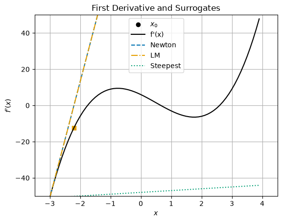
In this case, do we expect the Newton and LM steps to be the same? Explain.
Why does increase with a steepest descent () step? I thought the main idea was that because is positive definite the step is in a descent direction!
Consider 
calc_step(0, 1e-2)x0 = 0
f(x0) = 1.5
f'(x0) = 6
f''(x0) = -8
### Newton Step ###
xN = 0.75
pN = xN - x0 = 0.75
f(xN) = 3.486328125
f(xN) - f(x0) = 1.986328125
### Levenberg-Marquardt Step ###
xLM = -600.0
pLM = xLM - x0 = -600.0
f(xLM) = 65014556401.5
f(xLM) - f(x0) = 65014556400.0
### Steepest Descent Step ###
xSD = -6.0
pSD = xSD - x0 = -6.0
f(xSD) = 685.5
f(xSD) - f(x0) = 684.0
Discussion
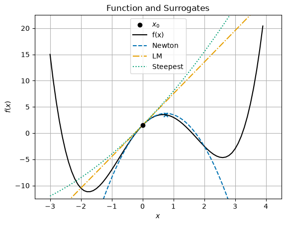
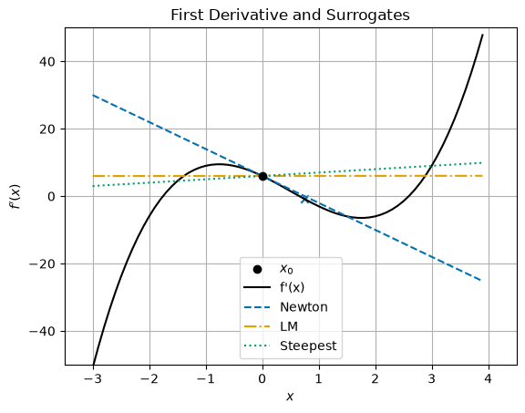
Why does increase for all of the steps?
Explain Newton-type method in the context of root finding for using the second plot.
Descent Properties
Line Search
Excerpts from Section 3.4 in Biegler (2010).
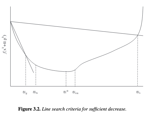
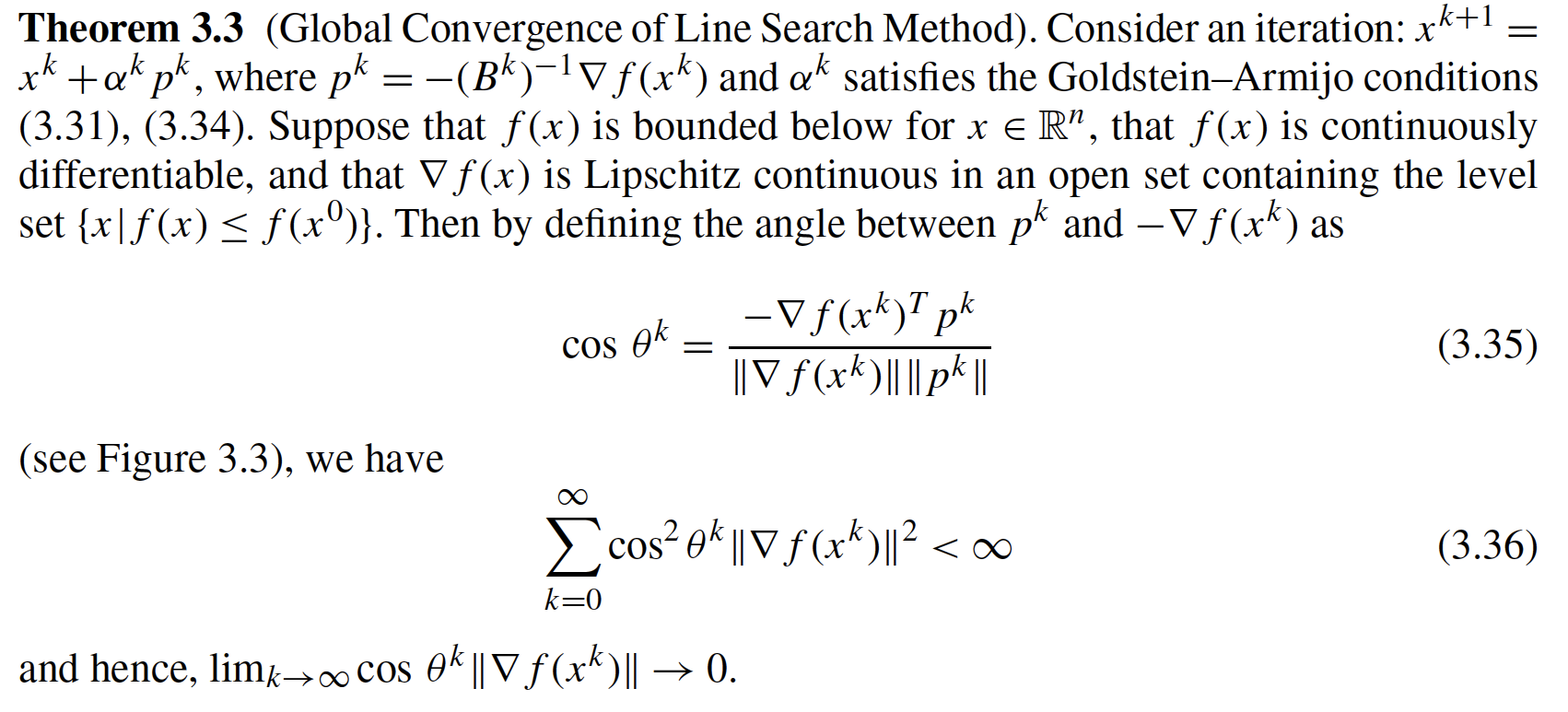
The Wolfe conditions require that (3.31) be satisfied as well as
for . From Figure 3.2, we see that satisfies these conditions.
The strong Wolfe conditions are more restrictive and require satisfaction of
for . From Figure 3.2, we see that satisfies these conditions.
The Goldstein or Goldstein–Armijo conditions require that (3.31) be satisfied as well as
Visualization Code
The line search conditions, as one picture
![Armijo and Goldstein conditions for steepest descent from x^k=-3: the accepted step lengths are the interval [\alpha_g, \alpha_a] where the function value stays below the Armijo line and above the Goldstein line.](/optimization/build/eb19b57463aecb83e9e175e2d11e404f.png)
This is Biegler Figure 3.2 for our test function. It is rendered from
figures/plots/line-search-conditions.py and is the same image printed in the course
pack, so what you annotate in lecture and what you see here cannot drift apart.
The cells below are the live version: plot_alpha redraws this for any , any
algorithm and any , so you can explore cases the static figure does not
cover -- including one where the line search fails.
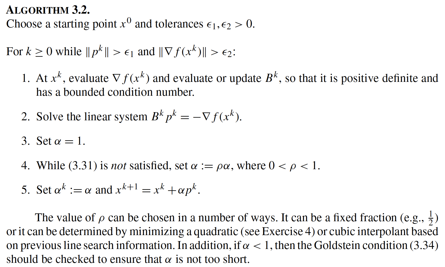
Goal: Visualize Armijo and Goldstein conditions for an example.
def plot_alpha(xk, eta_ls=0.25, algorithm="newton", alpha_max=1.0):
    """
    Calculate step and visualize line search conditions

    Arguments:
        xk : initial point (required)
        eta_ls : eta in Goldstein-Armijo conditions
        algorithm : either "newton" or "steepest-descent"
        alpha_max : plots alpha between 0 and alpha_max

    Returns:
        Nothing

    Creates:
        Plot showing function value and line search conditions as a function of alpha
    """

    fxk = f(xk)
    dfxk = df(xk)

    if algorithm == "newton":
        pk = -dfxk / ddf(xk)
    elif algorithm == "steepest-descent":
        pk = -dfxk
    else:
        raise ValueError(
            "algorithm argument must be either 'newton' or 'steepest-descent'"
        )

    print("Considering xk =", xk, "and f(xk) = ", fxk)
    print("Step with", algorithm, "algorithm:")
    print("pk = ", pk)
    print("With full step, xk+1 =", pk + xk, "and f(xk+1) =", f(xk + pk))

    n = 100
    alpha = np.linspace(0, alpha_max, n)
    fval = np.zeros(n)

    for i in range(0, n):
        fval[i] = f(xk + alpha[i] * pk)

    fs = 18
    plt.figure()

    # Evaluate f(x^{k+1}) for different alpha values.
    # Colour and linestyle match figures/plots/line-search-conditions.py, the
    # static version of this figure in the course pack: house cycle in order,
    # black solid, blue dashed, orange dash-dot. The linestyles are what make
    # the three series separable in greyscale.
    plt.plot(alpha, fval, color="black", linestyle="-", label=r"$f(x^{k+1})$")

    # Armijo condition
    arm = np.zeros(n)
    for i in range(0, n):
        arm[i] = fxk + eta_ls * alpha[i] * dfxk * pk

    plt.plot(alpha, arm, color="#0072B2", linestyle="--", label="Armijo")

    # Goldstein condition
    gold = np.zeros(n)
    for i in range(0, n):
        gold[i] = fxk + (1 - eta_ls) * alpha[i] * dfxk * pk

    plt.plot(alpha, gold, color="#E69F00", linestyle="-.", label="Goldstein")

    # Apply backtracking linestep (starting with alpha = alpha_max)
    i = n - 1
    flag = True
    failed = False
    while flag:

        if i < n - 1 and fval[i] < gold[i]:
            flag = False
            print(
                "Line search failed. Goldstein conditions violated. Consider increasing alpha_max."
            )
            failed = True

        # Armijo condition
        if fval[i] < arm[i]:
            flag = False
        else:
            i = i - 1

        if i < 0:
            print("Line search failed. Try decreasing alpha_max.")
            failed = True
            # Stop here. Without this, the loop keeps going with a negative
            # index, which wraps around to the end of the array and reports a
            # second, contradictory diagnosis.
            flag = False

    if not failed:
        print(
            "alphak =",
            alpha[i],
            "with backtracking line search starting at alpha =",
            alpha_max,
        )
        print("f(xk + alphak*pk) =", fval[i])

        plt.scatter(
            alpha[i],
            fval[i],
            marker="x",
            color="black",
            label=r"$\alpha^{k}$ for line search",
        )

    # Labels
    plt.xlabel(r"$\alpha^k$", fontsize=fs)
    plt.ylabel(r"$f(x^k + \alpha^k p^k)$", fontsize=fs)
    plt.grid()
    plt.legend()
    plt.show()
Newton Step, 
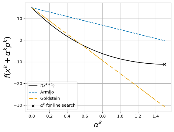
plot_alpha(-3, eta_ls=0.25, algorithm="newton", alpha_max=1.5)Considering xk = -3 and f(xk) = 15.0
Step with newton algorithm:
pk = 0.796875
With full step, xk+1 = -2.203125 and f(xk+1) = -8.660857647657394
alphak = 1.5 with backtracking line search starting at alpha = 1.5
f(xk + alphak*pk) = -11.1743426900357
Discussion
Why did the backtracking line search stop at
alpha_max?Is it possible to find a larger improvement in with ?
Steepest Descent Step, 
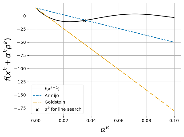
plot_alpha(-3, eta_ls=0.25, algorithm="steepest-descent", alpha_max=1e-1)Considering xk = -3 and f(xk) = 15.0
Step with steepest-descent algorithm:
pk = 51
With full step, xk+1 = 48 and f(xk+1) = 2534689.5
alphak = 0.03535353535353535 with backtracking line search starting at alpha = 0.1
f(xk + alphak*pk) = -8.67145500733185
Discussion
Why did the line search stop where the Armijo conditions are satisfied?
Why not further decrease to achieve a greater improvement in the objective?
Newton Step, 
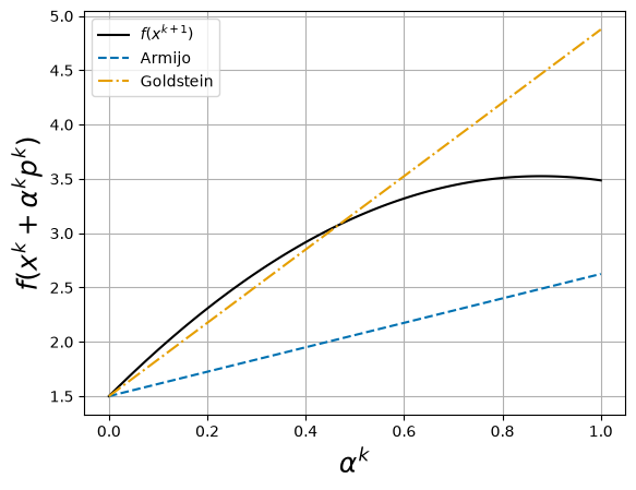
plot_alpha(0, eta_ls=0.25, algorithm="newton", alpha_max=1.0)Considering xk = 0 and f(xk) = 1.5
Step with newton algorithm:
pk = 0.75
With full step, xk+1 = 0.75 and f(xk+1) = 3.486328125
Line search failed. Goldstein conditions violated. Consider increasing alpha_max.
Discussion
Why does the line search fail?
How could we modify Newton’s method to improve robustness?
Steepest Descent Step, 
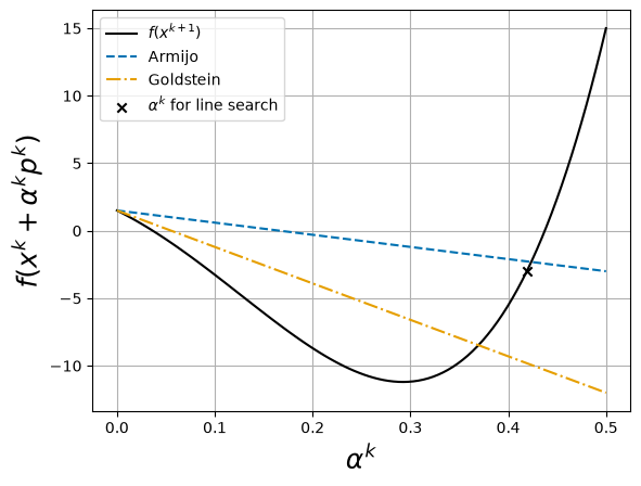
plot_alpha(0, eta_ls=0.25, algorithm="steepest-descent", alpha_max=5e-1)Considering xk = 0 and f(xk) = 1.5
Step with steepest-descent algorithm:
pk = -6
With full step, xk+1 = -6 and f(xk+1) = 685.5
alphak = 0.4191919191919192 with backtracking line search starting at alpha = 0.5
f(xk + alphak*pk) = -2.9749848430038526
Discussion
How does the region where the Armijo and Goldstein conditions are satisfied change for different values of
eta_ls?
Trust Regions
Excerpts from Section 3.5 in Biegler (2010).
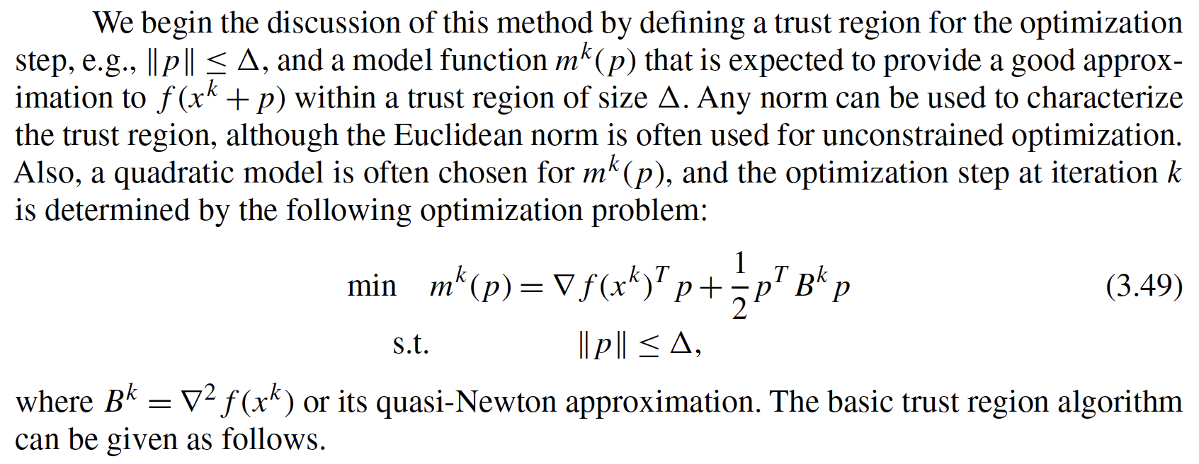
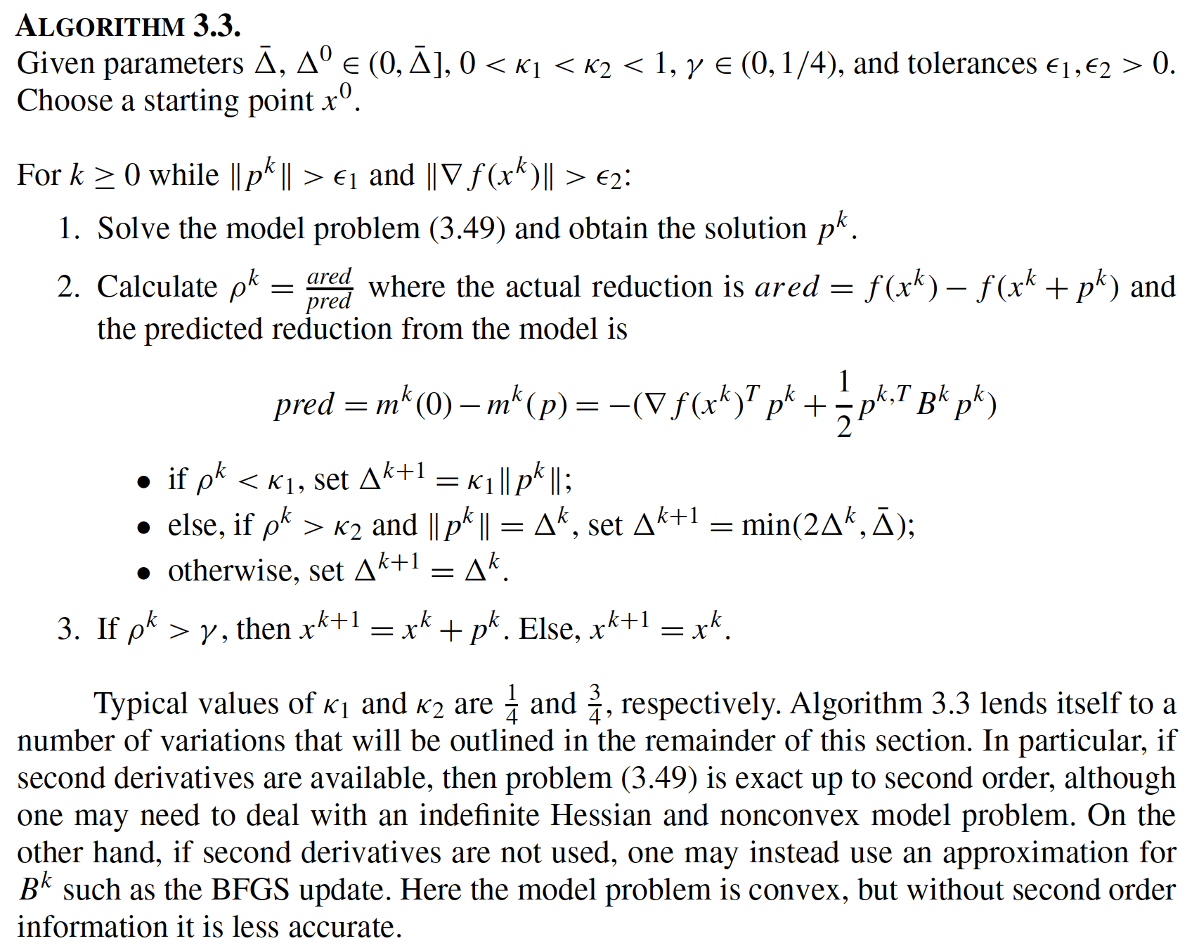
Main Idea and General Algorithm
Trust Region Variations
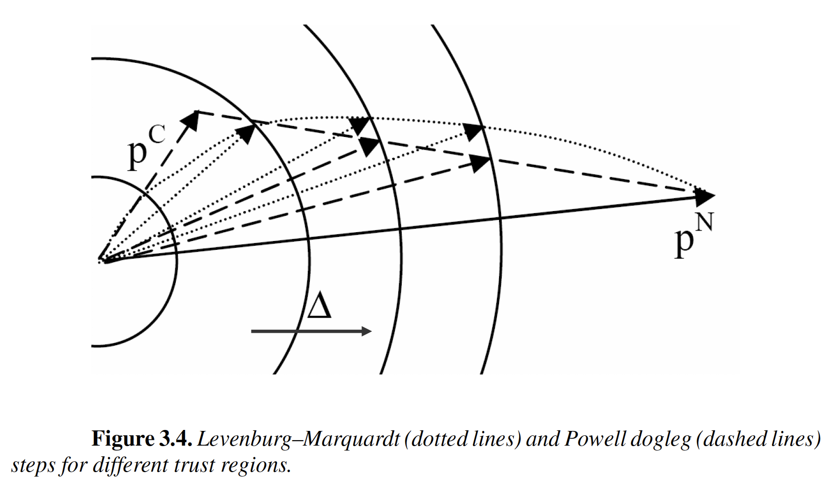
: Cauchy step
: Newton step
Levenberg-Marquardt
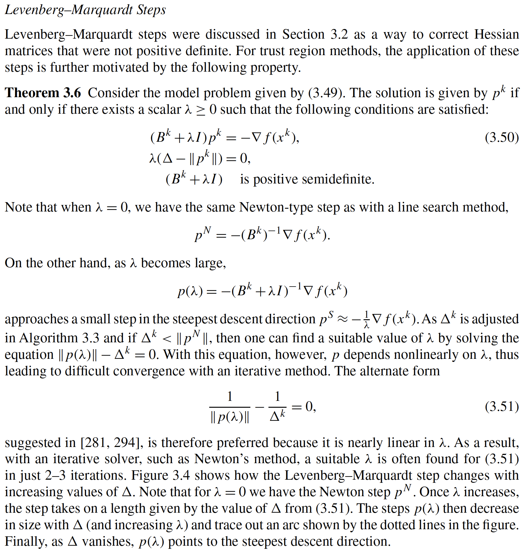
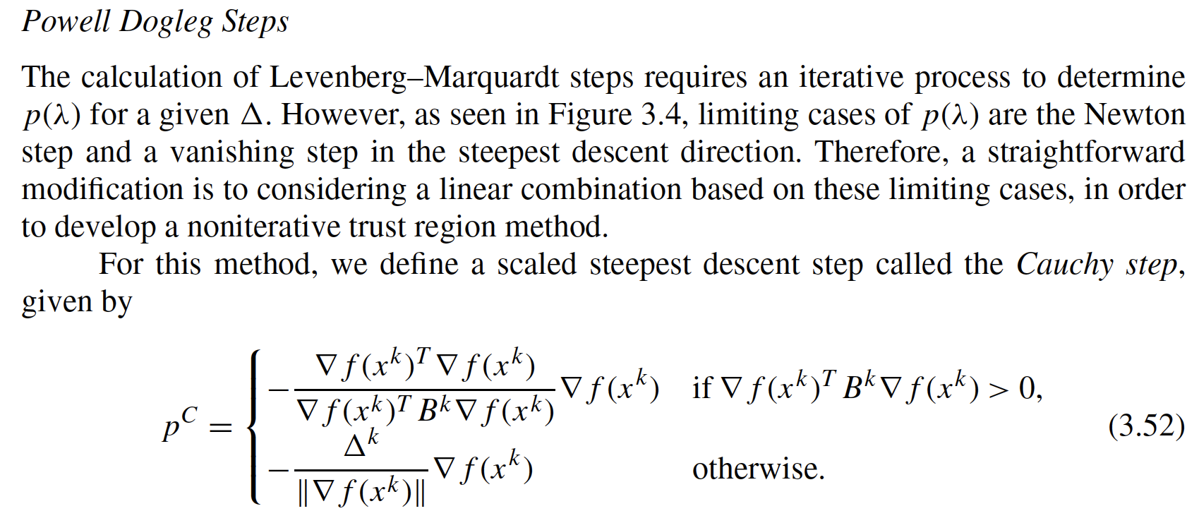
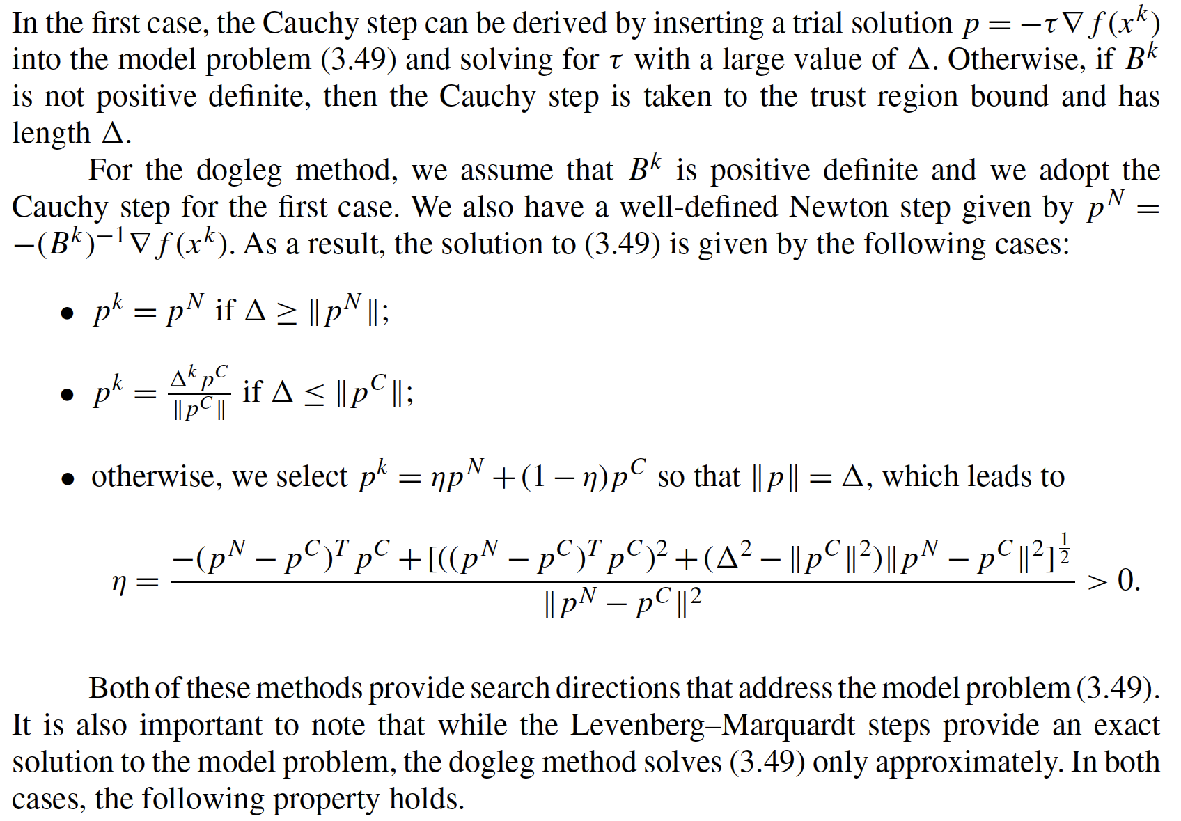
Powell Dogleg