This notebook contains material from cbe67701-uncertainty-quantification; content is available on Github.
7.2 Latin Hypercube Sampling
Created by V.Vijay Kumar Naidu (vvelagal@nd.edu)
The text, examples, and codes in this notebook were adapted from the following references:
- https://en.wikipedia.org/wiki/Latin_hypercube_sampling
- McClarren, Ryan G (2018). Uncertainty Quantification and Predictive Computational Science: A Foundation for Physical Scientists and Engineers, Chapter 7 : Sampling-Based Uncertainty Quantification Monte Carlo and Beyond, Springer, https://link.springer.com/chapter/10.1007%2F978-3-319-99525-0_7
# Install Python libraries
!pip install -q sobol_seq
!pip install -q ghalton
!pip install -q pyDOE
# Import
import matplotlib.pyplot as plt
import numpy as np
import scipy.sparse as sparse
import scipy.sparse.linalg as linalg
import scipy.integrate as integrate
import math
from scipy.stats.distributions import norm
from scipy.stats import gamma
import sobol_seq
import ghalton
from scipy import stats
from pyDOE import *
%matplotlib inline
# Download figures (if needed)
import os, requests, urllib

# GitHub pages url
url = "https://ndcbe.github.io/cbe67701-uncertainty-quantification/"

# relative file paths to download
# this is the only line of code you need to change
file_paths = ['figures/lhs_custom_distribution.png', 'figures/chapter7-screenshot.PNG']

# loop over all files to download
for file_path in file_paths:
    print("Checking for",file_path)
    # split each file_path into a folder and filename
    stem, filename = os.path.split(file_path)

    # check if the folder name is not empty
    if stem:
        # check if the folder exists
        if not os.path.exists(stem):
            print("\tCreating folder",stem)
            # if the folder does not exist, create it
            os.mkdir(stem)
    # if the file does not exist, create it by downloading from GitHub pages
    if not os.path.isfile(file_path):
        file_url = urllib.parse.urljoin(url,
                urllib.request.pathname2url(file_path))
        print("\tDownloading",file_url)
        with open(file_path, 'wb') as f:
            f.write(requests.get(file_url).content)
    else:
        print("\tFile found!")
7.2.1 Latin Hypercube Basics
Latin hypercube sampling (LHS) is a statistical method for generating a near random samples with equal intervals.
To generalize the Latin square to a hypercube, we define a X = (X1, . . . , Xp) as a collection of p independent random variables. To generate N samples, we divide the domain of each Xj in N intervals. In total there are Np such intervals. The intervals are defined by the N + 1 edges:
7.2.1.1 Latin Hypercube in 2D
Makes a Latin Hyper Cube sample and returns a matrix X of size n by 2. For each column of X, the n values are randomly distributed with one from each interval (0,1/n), (1/n,2/n), ..., (1-1/n,1) and they are randomly permuted.
def latin_hypercube_2d_uniform(n):
    lower_limits=np.arange(0,n)/n
    upper_limits=np.arange(1,n+1)/n

    points=np.random.uniform(low=lower_limits,high=upper_limits,size=[2,n]).T
    np.random.shuffle(points[:,1])
    return points
n=20
p=latin_hypercube_2d_uniform(n)
plt.figure(figsize=[5,5])
plt.xlim([0,1])
plt.ylim([0,1])
plt.scatter(p[:,0],p[:,1],c='r')

for i in np.arange(0,1,1/n):
    plt.axvline(i)
    plt.axhline(i)
plt.show

7.2.1.2 Latin-hypercube designs can be created using the following simple syntax
The following is adapted from:https://pythonhosted.org/pyDOE/randomized.html.
lhs(n, [samples, criterion, iterations])n: an integer that designates the number of factors (required).
samples: an integer that designates the number of sample points to generate for each factor (default: n) criterion: a string that tells lhs how to sample the points (default: None, which simply randomizes the points within the intervals):
“center” or “c”: center the points within the sampling intervals “maximin” or “m”: maximize the minimum distance between points, but place the point in a randomized location within its interval
“centermaximin” or “cm”: same as “maximin”, but centered within the intervals
“correlation” or “corr”: minimize the maximum correlation coefficient
The output design scales all the variable ranges from zero to one which can then be transformed as the user wishes (like to a specific statistical distribution using the scipy.stats.distributions ppf (inverse cumulative distribution) function
from scipy.stats.distributions import norm
from pyDOE import *
lhd = lhs(2, samples=5)
lhd = norm(loc=0, scale=1).ppf(lhd)  # this applies to both factors here
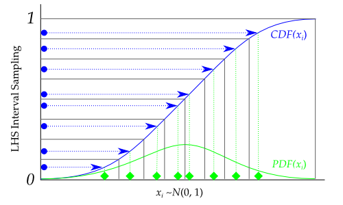
Graphically, each transformation would look like the following, going from the blue sampled points (from using lhs) to the green sampled points that are normally distributed: (Adapted from https://pythonhosted.org/pyDOE/randomized.html)
An example for Latin-Hyper cube sampling
design = lhs(4, samples=10)
from scipy.stats.distributions import norm
means = [1, 2, 3, 4]
stdvs = [0.1, 0.5, 1, 0.25]
for i in range(4):
    design[:, i] = norm(loc=means[i], scale=stdvs[i]).ppf(design[:, i])

design
7.2.2 Advection-Diffusion-Reaction (ADR) Example
7.2.2.1 Set up diffusion reaction equation
The steady advection-diffusion-reaction(ADR) equation in one-spatial dimension with a spatially constant, but uncertain, diffusion coefficient, a linear reaction term, and a prescribed uncertain source.
$$ \nu \frac{du}{dx} - \omega \frac{d^2u}{dx^2} + \kappa(x)u = S(x) $$The QoI is total reaction rate:$$ Q= \int^{10}_{0} \kappa(x_ u)u(x)dx $$ where v and ω are spatially constant with means $$ \nu = 10, μ_{ω} = 20, $$ and $$ Var(v) = 0.0723493, Var(ω) = 0.3195214. $$
The reaction coefficient, κ(x), is given by $$ κ(x) = κ_{l} \space x ∈ (5, 7.5) $$ $$ \space κ_{h} \space otherwise$$
The value of the source is given by $$S(x) = qx(10 − x),$$
def ADRSource(Lx, Nx, Source, omega, v, kappa):
    #Solves the diffusion equation with Generalized Source
    A = sparse.dia_matrix((Nx,Nx),dtype="float")
    dx = Lx/Nx
    i2dx2 = 1.0/(dx*dx)
    #fill diagonal of A
    A.setdiag(2*i2dx2*omega + np.sign(v)*v/dx + kappa)
    #fill off diagonals of A
    A.setdiag(-i2dx2*omega[1:Nx] +
              0.5*(1-np.sign(v[1:Nx]))*v[1:Nx]/dx,1)
    A.setdiag(-i2dx2*omega[0:(Nx-1)] -
              0.5*(np.sign(v[0:(Nx-1)])+1)*v[0:(Nx-1)]/dx,-1)
    #solve A x = Source
    Solution = linalg.spsolve(A.tocsr(),Source)
    Q = integrate.trapz(Solution*kappa,dx=dx)
    return Solution, Q
Solve diffusion equation
Lx = 10
Nx = 2000
dx = Lx/Nx
Source_func = lambda x, q:  q*x*(10-x)
kappa_func = lambda x, kappal, kappah: kappah + (kappal-kappah)*(x>5)*(x<7.5)
v_func = lambda x,v: v*np.ones(x.size)
omega_func = lambda x,omega: omega*np.ones(x.size)

#nominal values

import csv

xs = np.linspace(dx/2,Lx-dx/2,Nx)
source = Source_func(xs, 1)
kappa = kappa_func(xs, 0.1, 2)

omega_nom = 20
omega_var = 0.3195214
v_nom = 10
v_var = 0.0723493
kappal_nom = 0.1
kappal_var = 8.511570e-6
kappah_nom = 2
kappah_var = 0.002778142
q_nom = 1
q_var = 7.062353e-4
vs = v_func(xs, v_nom)
print(vs)
sol,Q = ADRSource(Lx, Nx, source, omega_func(xs, omega_nom), vs, kappa)
print(Q)
plt.plot(xs,sol)
plt.show()

We are going to join gamma RVs with a normal copula. First we get the normal samples
means = [v_nom, omega_nom, kappal_nom, kappah_nom, q_nom]
varmat = np.zeros((5,5))
#fill in diagonal
corrmat = np.ones((5,5))
corrmat[0,:] = (1,.1,-0.05,0,0)
corrmat[1,:] = (.1,1,-.4,.3,.5)
corrmat[2,:] = (-0.05,-.4,1,.2,0)
corrmat[3,:] = (0,.3,0.2,1,-.1)
corrmat[4,:] = (0,.5,0,-.1,1)
print(corrmat-corrmat.transpose())
print(corrmat)


varmat[np.diag_indices(5)] = [v_var, omega_var, kappal_var, kappah_var, q_var]
for i in range(5):
    for j in range(5):
        varmat[i,j] = math.sqrt(varmat[i,i])*math.sqrt(varmat[j,j])*corrmat[i,j]
print(varmat)
print(varmat-varmat.transpose())
print(np.linalg.eig(varmat))

# Warning: choosing a large number here will make the notebook take a long time
# to solve.
# samps = 10**6
samps = 10**4
# samps = 10**3
test = norm.cdf(np.random.multivariate_normal(np.zeros(5), corrmat, samps))

print(np.max(test[:,0]))
import tabulate
#print(tabulate.tabulate(corrmat, tablefmt="latex", floatfmt=".2f"))
The distributions will be gammas
def gen_samps(samps,test):
    #v will have v_nom = 10 v_var = 1 which makes alpha = 10 beta = 10 or theta = 1/10
    vsamps = gamma.ppf(test[:,0], a = 100, scale = 1/10)
    #print(np.mean(vsamps), np.var(vsamps), np.std(vsamps))
    #plt.hist(vsamps)

    #omega will have  omega_nom = 20, var = 4 which makes alpha = 100 beta = 5, theta = 1/5
    omegasamps = gamma.ppf(test[:,1], a = 100, scale = 1/5)
    #print(np.mean(omegasamps), np.var(omegasamps), np.std(omegasamps))
    #plt.hist(omegasamps)

    #kappa_l will have kappa_l = 0.1 var = (0.01)^2 this makes alpha = 100 and theta = 1/1000
    kappalsamps = gamma.ppf(test[:,2], a = 100, scale = 1/1000)
    #print(np.mean(kappalsamps), np.var(kappalsamps), np.std(kappalsamps))
    #plt.hist(kappalsamps)

    #kappa_h will have kappa_h = 2 var = .04 this makes alpha = 100 and theta = 1/50
    kappahsamps = (test[:,3]>0.005)*(1.98582-4.82135) + (4.82135) # #gamma.ppf(test[:,3], a = 100, scale = 1/50)
    print(np.mean(kappahsamps), np.var(kappahsamps), np.std(kappahsamps))
    #plt.hist(kappahsamps)

    #q will have q = 1 var = 0.01 this makes alpha = 100 and theta = 1/100
    qsamps = gamma.ppf(test[:,4], a = 100, scale = 1/100)
    #print(np.mean(qsamps), np.var(qsamps),np.std(qsamps))
    #plt.hist(qsamps)

    return vsamps,omegasamps,kappalsamps,kappahsamps,qsamps
vsamps,omegasamps,kappalsamps,kappahsamps,qsamps = gen_samps(samps,test)

var_list = [vsamps,omegasamps,kappalsamps,kappahsamps,qsamps]
cormat_emp = np.zeros((5,5))
tmp = np.vstack((var_list[0],var_list[1],var_list[2],var_list[3],var_list[4]))
cormat_emp = np.cov(tmp)
sens = np.array([-1.74063875491,-0.970393472244,13.1587256647,17.7516305655,52.3902556893])
print(cormat_emp, np.dot(sens,np.dot(cormat_emp,sens)))
Qs = np.zeros(samps)
print(np.mean(vsamps),np.mean(omegasamps),np.mean(kappalsamps), np.mean(kappahsamps),np.mean(qsamps))
for i in range(samps):
    sol,Qs[i] = ADRSource(Lx, Nx, Source_func(xs, qsamps[i]), omega_func(xs, omegasamps[i]), v_func(xs, vsamps[i]),
                          kappa_func(xs, kappalsamps[i], kappahsamps[i]))
plt.hist(kappahsamps)
plt.show()
plt.hist(Qs)
plt.show()
print(np.mean(Qs),stats.scoreatpercentile(Qs,95) ,stats.scoreatpercentile(Qs,5),np.std(Qs), stats.kurtosis(Qs), stats.skew(Qs))
Qref = Qs.copy()
np.savetxt(fname="ref_"+ str(samps) + "_binomial.csv", delimiter=",", X=Qref)


Now we will do 100 samples and compare
samps = 100 #4*10**4
print (samps)
test = norm.cdf(np.random.multivariate_normal(np.zeros(5), corrmat, samps))
vsamps,omegasamps,kappalsamps,kappahsamps,qsamps = gen_samps(samps,test)
QSRS = np.zeros(samps)
for i in range(samps):
    sol,QSRS[i] = ADRSource(Lx, Nx, Source_func(xs, qsamps[i]), omega_func(xs, omegasamps[i]), v_func(xs, vsamps[i]),
                          kappa_func(xs, kappalsamps[i], kappahsamps[i]))
plt.hist(QSRS)
plt.show()
print(np.mean(QSRS),stats.scoreatpercentile(QSRS,95),stats.scoreatpercentile(QSRS,5),np.std(QSRS),
      stats.kurtosis(QSRS), stats.skew(QSRS))

7.2.2.2 Apply LHS
#lhd will have the values in 0 to 1
lhd = lhs(5, samples=samps)
#now i need to turn these into samples from N(0,Corrmat)
#do cholesky fact
chol = np.linalg.cholesky(corrmat)

lhs_unif = np.zeros((samps,5))
for i in range(samps):
    lhs_unif[i,:] = np.dot(chol,norm.ppf(lhd[i,:]))
#print(lhs_unif)
#plt.plot(lhd[:,0],lhd[:,1],'.')
#plt.show()
plt.plot(lhs_unif[:,0],lhs_unif[:,1],'.')
plt.show()

test_lhs = norm.cdf(lhs_unif)

vsamps,omegasamps,kappalsamps,kappahsamps,qsamps = gen_samps(samps,test_lhs)
QLHS = np.zeros(samps)
for i in range(samps):
    sol,QLHS[i] = ADRSource(Lx, Nx, Source_func(xs, qsamps[i]), omega_func(xs, omegasamps[i]), v_func(xs, vsamps[i]),
                          kappa_func(xs, kappalsamps[i], kappahsamps[i]))
plt.hist(QLHS)
plt.show()
print(np.mean(QLHS),stats.scoreatpercentile(QLHS,95),stats.scoreatpercentile(QLHS,5),np.std(QLHS),
      stats.kurtosis(QLHS), stats.skew(QLHS))
print(np.mean(Qs),stats.scoreatpercentile(Qs,95) ,stats.scoreatpercentile(Qs,5),np.std(Qs), stats.kurtosis(Qs), stats.skew(Qs))

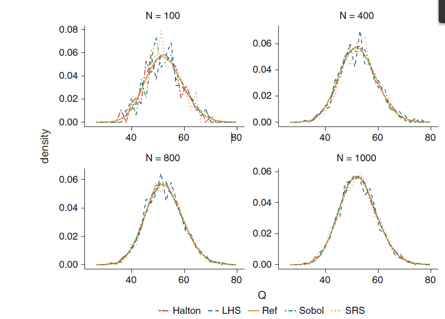
Below is Figure 7.13 in McClarren (2018); it shows the convergence rates of different methods compared against a LHS with 10$^6$ samples.