This notebook contains material from cbe67701-uncertainty-quantification; content is available on Github.
7.1 Latin Hypercube and Quasi-Monte Carlo Sampling
Created by Dezhao Huang (dhuang2@nd.edu)
These examples and codes were adapted from:
- https://risk-engineering.org/notebook/monte-carlo-LHS.html
- McClarren, Ryan G (2018). Uncertainty Quantification and Predictive Computational Science: A Foundation for Physical Scientists and Engineers, Chapter 7 : Sampling-Based Uncertainty Quantification Monte Carlo and Beyond, Springer, https://link.springer.com/chapter/10.1007%2F978-3-319-99525-0_7
Chapter 7 Overview
- Basic Monte Carlo methods: maximum likelihood estimation and methods of moments
- Design based sampling: Latin Hypercube Sampling
- Quasi-Monte Carlo: Halton sequences and Sobol sequence
# Load libraries
import math
import numpy
import scipy.stats
import matplotlib.pyplot as plt
plt.style.use("bmh")
import sympy
from IPython.display import Image
from IPython.core.display import HTML
## Install missing packages
!pip install sobol_seq

import sobol_seq

!pip install pyDOE
from pyDOE import lhs
# Download figures (if needed)
import os, requests, urllib

# GitHub pages url
url = "https://ndcbe.github.io/cbe67701-uncertainty-quantification/"

# relative file paths to download
# this is the only line of code you need to change
file_paths = ['figures/LHS.png']

# loop over all files to download
for file_path in file_paths:
    print("Checking for",file_path)
    # split each file_path into a folder and filename
    stem, filename = os.path.split(file_path)

    # check if the folder name is not empty
    if stem:
        # check if the folder exists
        if not os.path.exists(stem):
            print("\tCreating folder",stem)
            # if the folder does not exist, create it
            os.mkdir(stem)
    # if the file does not exist, create it by downloading from GitHub pages
    if not os.path.isfile(file_path):
        file_url = urllib.parse.urljoin(url,
                urllib.request.pathname2url(file_path))
        print("\tDownloading",file_url)
        with open(file_path, 'wb') as f:
            f.write(requests.get(file_url).content)
    else:
        print("\tFile found!")
The simplest 1D integration problem,
$\int_1^5 x^2$
We can estimate this integral using a standard Monte Carlo method, where we use the fact that the expectation of a random variable is related to its integral
$\mathbb{E}(f(x)) = \int_I f(x) dx$
We will sample a large number $N$ of points in $I$ and calculate their average, and multiply by the range over which we are integrating.
# First, let's take a look at the analytical result:
result = {}
x = sympy.Symbol("x")
i = sympy.integrate(x**2)
result["analytical"] = float(i.subs(x, 5) - i.subs(x, 1))
print("Analytical result: {}".format(result["analytical"]))
Monte Carlo Simulator : $<F^N> = (b-a)\frac{1}{N}\sum_{i = 0}^{N-1} f(x_i)$
# Second, use the simple monte carlo method to calculate the integral
N = 1000
accum = 0
for i in range(N):
    x = numpy.random.uniform(1, 5)
    accum += x**2
interval_length = 5 - 1
result["MC"] = interval_length * accum / float(N)
print("Simple Monte Carlo result: {}".format(result["MC"]))
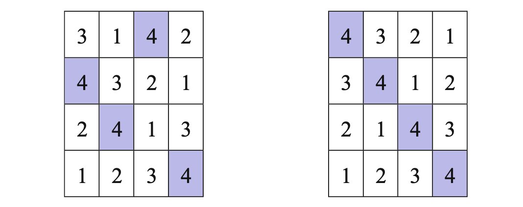
7.1.1 Latin hypercube sampling
Try to pick a design that fills the design space given a fixed number of samples.
The LHS figure below is from McClarren (2018).
N = 1000

seq = lhs(2, N)
accum = 0
for i in range(N):
    x = 1 + seq[i][0]*(5 - 1)
    y = 1 + seq[i][1]*(5**2 - 1**2)
    accum += x**2
volume = 5 - 1
result["LHS"] = volume * accum / float(N)
print("Latin hypercube result: {}".format(result["LHS"]))
7.1.2 Quasi MC: Halton’s low discrepency sequences
Quasi-Monte Carlo(QMC) simulation is the traditional MCS but using deterministic sequences.
A low discrepancy (or quasi-random) sequence is a deterministic mathematical sequence of numbers that has the property of low discrepancy. This means that there are no clusters of points and that the sequence fills space roughly uniformly. The Halton sequence is a low discrepancy sequence that has useful properties for pseudo-stochastic sampling methods (also called “quasi-Monte Carlo” methods).
def halton(dim: int, nbpts: int):
    h = numpy.full(nbpts * dim, numpy.nan)
    p = numpy.full(nbpts, numpy.nan)
    P = [2, 3, 5, 7, 11, 13, 17, 19, 23, 29, 31]
    lognbpts = math.log(nbpts + 1)
    for i in range(dim):
        b = P[i]
        n = int(math.ceil(lognbpts / math.log(b)))
        for t in range(n):
            p[t] = pow(b, -(t + 1))
        for j in range(nbpts):
            d = j + 1
            sum_ = math.fmod(d, b) * p[0]
            for t in range(1, n):
                d = math.floor(d / b)
                sum_ += math.fmod(d, b) * p[t]

            h[j*dim + i] = sum_
    return h.reshape(nbpts, dim)
N = 1000
seq = halton(2, N)
plt.title("2D Halton sequence")
plt.scatter(seq[:,0], seq[:,1], marker=".", alpha=0.7);

N = 1000
plt.title("Simpling Random Sampling Sequence")
plt.scatter(numpy.random.uniform(size=N), numpy.random.uniform(size=N), marker=".", alpha=0.5);

seq = halton(2, N)
accum = 0
for i in range(N):
    x = 1 + seq[i][0]*(5 - 1)
    y = 1 + seq[i][1]*(5**2 - 1**2)
    accum += x**2
volume = 5 - 1
result["QMCH"] = volume * accum / float(N)
print("Quasi-Monte Carlo result (Halton): {}".format(result["QMCH"]))
Another quasi-random sequence commonly used for this purpose is the Sobol’ sequence. This equence was designed to make integral estiamtes on the p-dimensional hypercube converge as quickly as possible.
seq = sobol_seq.i4_sobol_generate(2, N)
plt.title("2D Sobol sequence")
plt.scatter(seq[:,0], seq[:,1], marker=".", alpha=0.5);

seq = sobol_seq.i4_sobol_generate(2, N)

accum = 0
for i in range(N):
    x = 1 + seq[i][0]*(5 - 1)
    y = 1 + seq[i][1]*(5**2 - 1**2)
    accum += x**2
volume = 5 - 1
result["QMCS"] = volume * accum / float(N)
print("Quasi-Monte Carlo result (Sobol): {}".format(result["QMCS"]))
7.1.3 Comparison (1 dimensional)
We can compare the error of our different estimates (each used the same number of runs):
for m in ["MC", "LHS", "QMCH", "QMCS"]:
    print("{:4} result: {:.8}  Error: {:E}".format(m, result[m], abs(result[m]-result["analytical"])))