A comprehensive reference for Integer Programming Algorithms: complete bound and cut proofs, numerical qualifications, and executable branch-and-bound/OA/GBD examples. The handout keeps the guided core; the reference supplies the longer arguments and calculations. Model data and source citations are retained.
Search size and feasible assignments¶
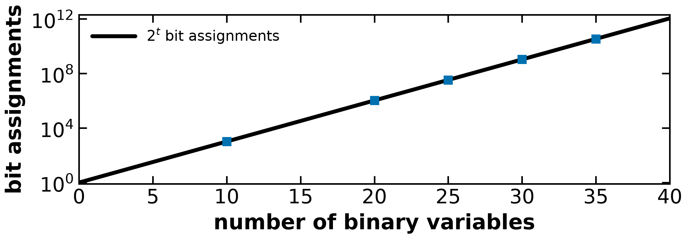
With binary variables there are bit assignments before constraints eliminate any of them. At an assumed 0.1 seconds per fixed-design LP, the counts for are 1024, , , and : approximately 102 seconds, 29.1 hours, 38.8 days, 3.40 years and 108.9 years. This is an illustrative enumeration cost, not a runtime prediction for branch and bound. BGW Appendix A, pp.758–760.
The integer-modeling reference owns the Sudoku formulation. Its indicators include nine per cell. Each supplied clue fixes one indicator to 1 and the other eight to 0. With 24 distinct clues, 216 indicators are fixed and 513 remain before row, column and box propagation. The naive assignments would take about years under the same assumed cost. Most are infeasible; call them assignments rather than solutions. Logical inference, presolve, relaxations and incumbent bounds avoid testing them all. They do not make every integer problem easy.
Relaxations, restrictions and global bounds¶
Let and retain the same objective. Then , including extended values for infeasible or unbounded problems. Every point of is available in , so minimizing over more points cannot increase the global value. No convexity is required for this inclusion argument. Conversely, a feasible point of a restriction is feasible in the original problem and supplies an upper bound for minimization, even if it was found by a local method.
A computed local minimum of a nonconvex relaxation need not be a lower bound. Convexity provides a useful sufficient condition for global continuous minimization; valid global underestimators can also supply bounds for nonconvex problems. The global-optimization reference owns spatial relaxations. General convexity and KKT proofs remain in Unconstrained Optimality and Multipliers.
Relaxing binary variables to preserves every original feasible binary design. An inactive deleted constraint does not establish identical returned coordinates when the optimizer is nonunique: with , different points can be optimal before and after deletion. In a convex problem, continuity and a segment argument can show that an optimum strictly inside a removed inequality remains optimal: a better relaxed point would give a nearby feasible point with smaller convex objective, a contradiction. Without convexity this implication fails. For , the optimum on has ; deleting the inactive bound admits a better optimum in . The two minimizers are approximately with value 0.099367, and with value -0.100617. The first point lies strictly inside the deleted bound, yet the second has lower cost. BGW Ch.15 p.513 distinguishes obtaining a global value from a local NLP solve.
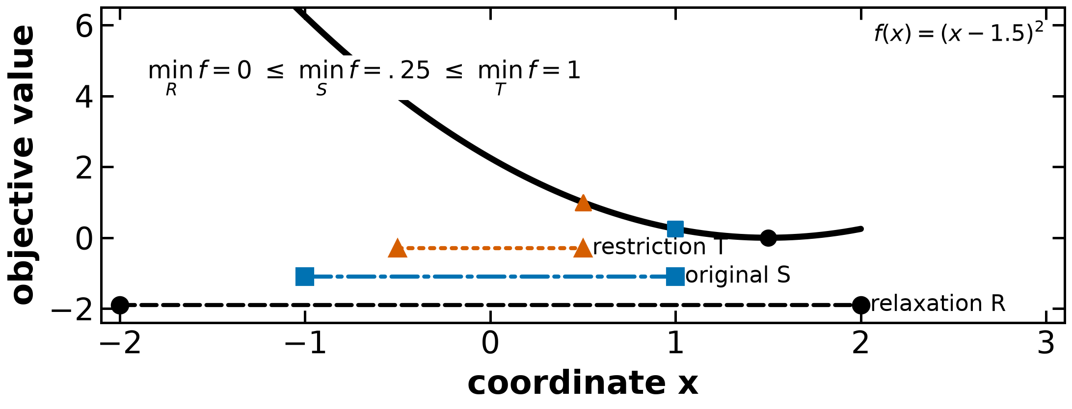
The lower interval bars mark domains, not objective values.
Branch and bound: algorithm and proof¶
A node restricts part of the integer domain. Its continuous relaxation contains every feasible integer descendant, so a certified node lower bound bounds that whole subtree. An incumbent is an original feasible integer design, with objective . To find one optimum:
Initialize a finite integer search domain, an active list and unless a feasible incumbent is known.
Select an active node and solve or bound its relaxation. Handle termination status before reading a solution.
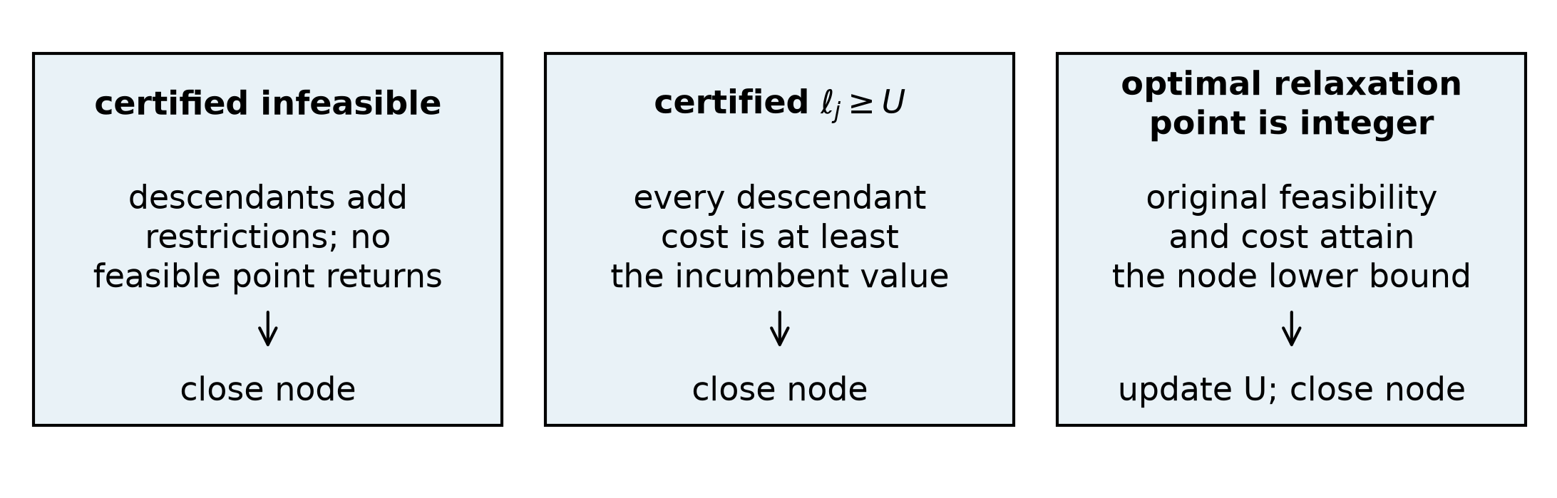
Close a certified infeasible node. Adding descendant restrictions cannot restore feasibility.
Close a node with . Every descendant objective is at least , so none improves the incumbent.
If an optimal relaxation point is integer and original-feasible, update the incumbent. Its objective attains the node lower bound; descendants cannot improve it.
Otherwise branch on a fractional integer variable, partitioning its domain into exhaustive disjoint children. Continue until no active subtree can improve or a declared limit is reached.
For a binary variable the children fix 0 or 1. General integer branching uses and . A finite binary domain gives a finite tree; LP solving and status certification are separate assumptions. An interrupted search returns an incumbent and a remaining bound, not automatic optimality. Unsolved children can inherit their parent’s lower bound when maintaining a global frontier bound.
The non-strict bound comparison is appropriate when finding one optimum. Enumerating every optimal design needs additional handling of tied bounds and optimal faces; closing an integral relaxation can hide other tied designs too. In numerical code, distinguish integer, feasibility and objective-gap tolerances, and check a rounded candidate in the original model. A relaxation can be unbounded without proving integer infeasibility; a solver limit or ambiguous infeasible-or-unbounded status is not a generic fathoming certificate. The MIPEX objective below is nonnegative, so unboundedness is impossible for that particular model. BGW §A.3.2 pp.759–761; Bonami et al. pp.187–188.
MIPEX: elimination, all nodes and the search tree¶
BGW p.760, problem MIPEX and Figure A.10, supplies
Because the coefficient of is positive and its lower expression is nonnegative on the relaxed box, an optimum has . Thus the reduced cost is . Coverage prices are per unit. For this one-row continuous covering model, buy available coverage first, then , then ; fixed variables contribute their fixed coverage and cost. This greedy property is specific to this fractional covering LP, not a general MILP algorithm.
The breadth-first sequence is:
| Node | Fixed coordinates | LP point | Value | Action |
|---|---|---|---|---|
| 1 | none | 5.8 | branch on | |
| 2 | 6 | branch on | ||
| 3 | 6.5 | branch on | ||
| 4 | infeasible | — | close | |
| 5 | 6.75 | branch on | ||
| 6 | infeasible | — | close | |
| 7 | 9 | incumbent 9 | ||
| 8 | infeasible | — | close | |
| 9 | 8 | incumbent 8 |
Nodes 4/5 descend from 2,6/7 from 3, and 8/9 from 5. Nine of the full tree’s 15 nodes are solved; only two of its eight fully specified leaves are visited. Rounding the root to gives coverage 8 rather than 9. Node 6 requires , immediately proving infeasibility. An early incumbent of 8 would close the node whose lower bound is 9, showing why traversal affects work. The final solution is , , objective 8. Full enumeration of all eight binary points independently confirms it. The MILP notebook gives separate node solves; the executable loop below owns the algorithm and shared tree figure.
Valid inequalities and the integer hull¶
A valid inequality holds at every feasible point of the original model, with its integer domains enforced. A separating cut additionally excludes the current relaxed point. For a nonempty bounded finite pure-integer set , is the smallest convex set containing it. Its vertices belong to . A linear objective therefore has an integer optimal vertex over this hull. The argument is an existence statement: a solver can return a fractional point of an optimal face. For example, every point on the segment between and minimizes the zero objective. For a linear objective on a bounded mixed-integer polyhedral feasible set, a minimizing hull vertex has integer designated coordinates; its continuous coordinates need not be integer. A fractional point on an optimal hull face may still be returned.
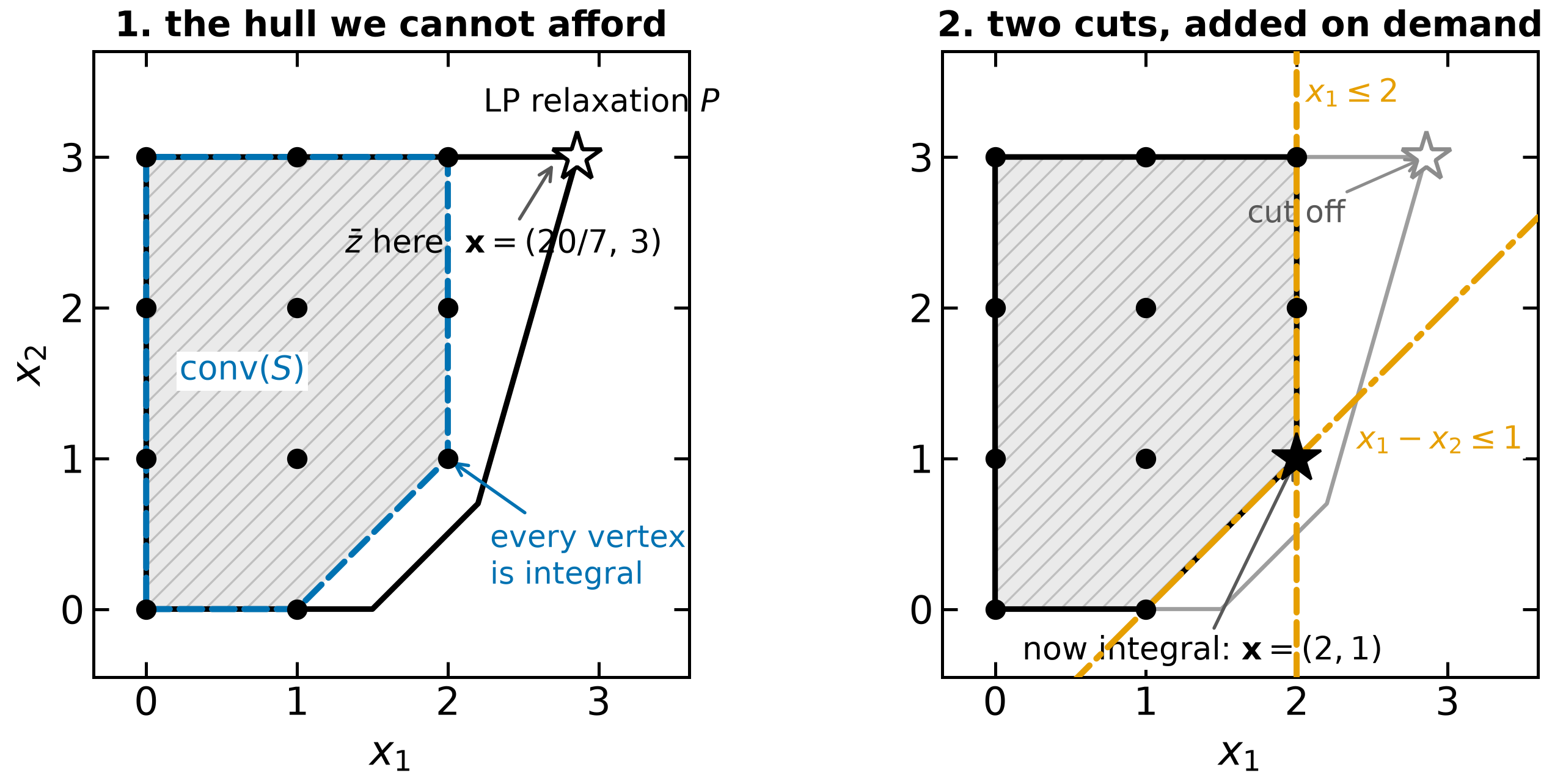
For the illustrated maximization, , the relaxation has , , , . Its optimum is with value . Every integer feasible point satisfies and . The first cut alone leaves optimum with value 7.5; both cuts give with value 7. Enumerating the integer points and all intersections verifies that the resulting polygon has vertices , exactly the integer hull. Equality with the hull is a property of this example, not a promised outcome after two cuts on general problems.
Hull facets may be numerous or difficult to describe. Useful cuts can instead come from recognized structures, disjunctions or tableau rows. Pairwise versus aggregated logic has its existing Logical Modeling home; a nonnegative aggregation can lose information even when every row remains valid.
Finite-hull proof. Any , with and , has . A minimizing point of the nonempty finite set attains that value. To obtain a vertex, among those minimizing points choose the smallest first coordinate, then the smallest second coordinate to break ties, and continue through all coordinates. If it were a nontrivial convex combination, every positive-weight member would first have to attain the same minimum cost. Coordinate-by-coordinate minimality would then force every such member to equal the chosen point. Thus it is a hull vertex belonging to . For a bounded mixed-integer linear model, each fixed integer assignment has a compact polytope. The mixed-integer hull is the hull of the finite union of those polytopes’ vertices; the same argument gives a minimizing vertex with the designated integer coordinates intact.
Pure fractional cuts, mixed rows and numerical care¶
For a simplex row with all variables nonnegative integers, write . Then is integer and no larger than , hence no larger than . Subtracting this integer part from the original equality yields
At a fractional basic solution, nonbasic variables are zero and , so this cuts off that relaxed point while retaining every integer feasible row solution. Floors, including those of negative coefficients, matter.
For , the pure fractional cut is ; the integer point satisfies it. If is continuous, the original row also permits , which that same cut wrongly removes. Mixed-integer rounding therefore requires a different derivation; blindly flooring a mixed row is invalid. Indeed, and , while only the first satisfies the proposed cut.
Branch-and-cut combines bound-based search with valid inequalities. Globally valid cuts can apply throughout the tree; cuts whose validity uses node bounds are local to that subtree. Cut selection, scaling and tolerances affect numerical behavior. Two nearly dependent rows can already be ill conditioned; limiting the number of cut rounds is not a conditioning theorem. Pure cutting-plane algorithms and extended cutting-plane MINLP methods also exist. Do not infer that a specific solve generated cuts merely because its backend can do so: a model may finish in presolve, and the continuous MIPEX node problems are LPs. Bonami et al. pp.187–188,191–192 discusses the branch-and-cut/OA framework. General near-rank/inertia examples remain in Math Primer.
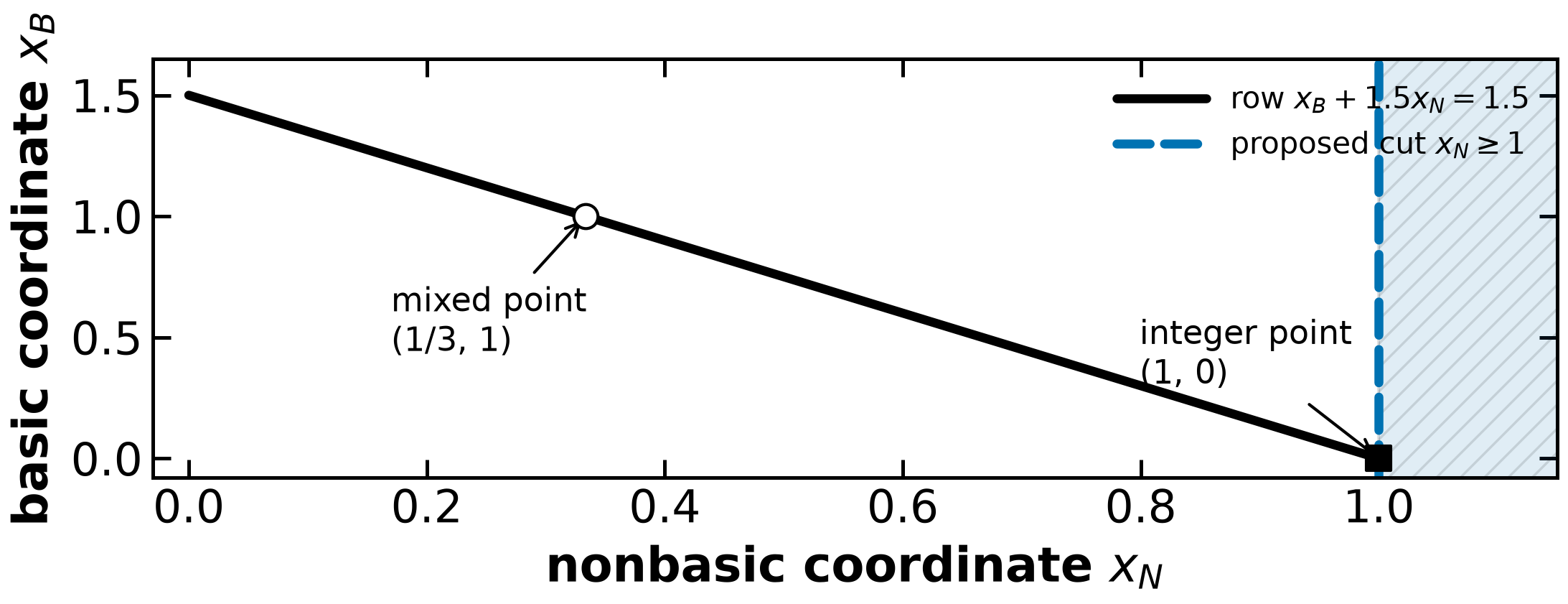
The plotted coordinate order is (x_N, x_B): nonbasic horizontally and basic vertically.
Convex MINLP and the fixed-design subproblem¶
Use the simplified problem
where is a nonempty compact polyhedral continuous domain and includes the pure-binary logic. Assume differentiable convex and each on the relevant domain. Retained equalities here are affine; arbitrary nonlinear equality tangents are not automatically outer relaxations. BGW §A.3.4 pp.763–766 treats a broader equality-relaxation variant with extra conditions; do not transfer its guarantee unchanged to a general equality model.
Fixing a permitted binary design gives a continuous restriction. Every original-feasible point of it supplies an upper bound, even without global optimality. A solver’s returned point must satisfy the original bounds/coupling rows, not only relaxed numerical bounds. A globally solved subproblem gives its design value . Certified lower and feasible upper values are needed if it is solved only approximately.
Normalize row units/scales before comparing them through a common violation variable. A common phase-I problem is
For at least one continuous finite row, compact nonempty makes the maximum violation attain a finite minimum. A globally certified proves the fixed design infeasible; a point with proves feasibility. A positive trial does not prove infeasibility. For on , the trial has violation 1 while has violation−1. On unbounded with , the free-scalar phase I is unbounded below despite feasibility. A nonnegative slack variant reports minimum 0 for feasible designs instead; distinguish these definitions. Nonlinear solver failure is not a phase-I certificate.
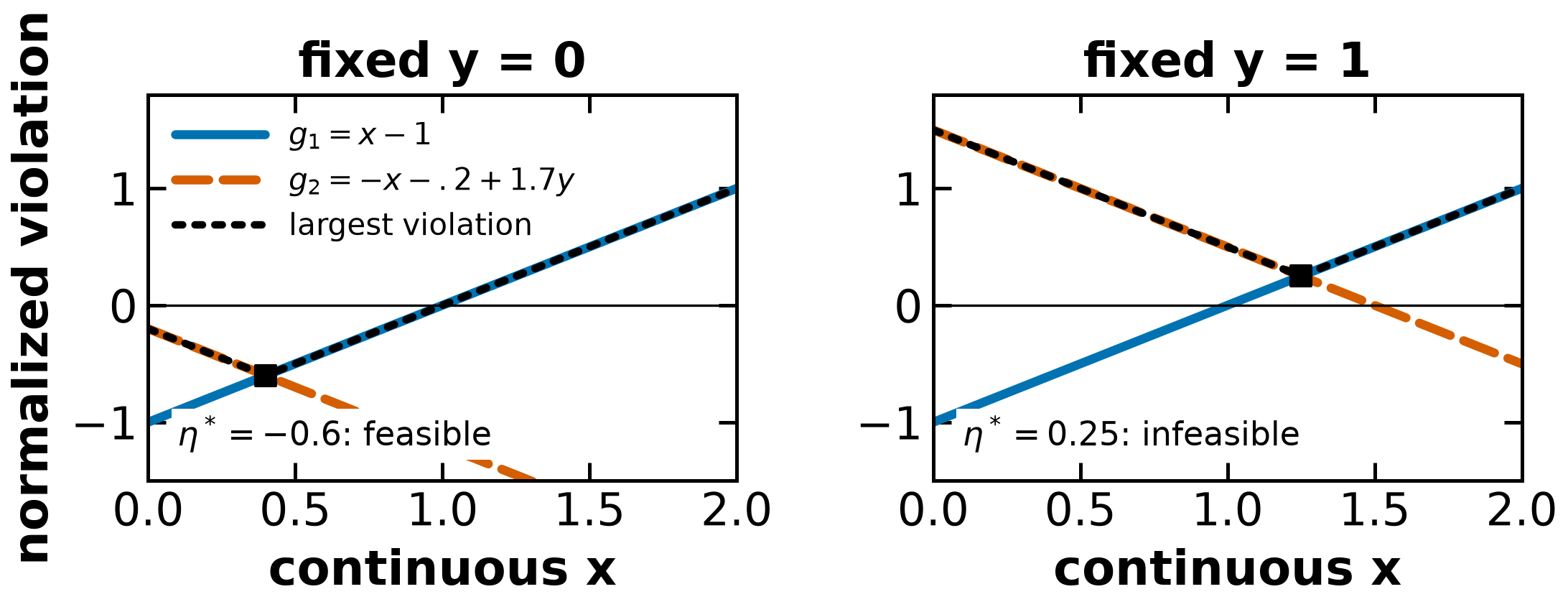
For the supplied affine rows, the global phase-I minimum is negative at y = 0 and positive at y = 1.
The broader BGW equality-relaxation variant¶
BGW pp.764–766 treats a broader model with nonlinear equalities, separate nonlinear inequalities, affine continuous rows and affine binary couplings:
For an equality-feasible linearization point and the course convention with Lagrangian term , form the diagonal direction matrix . The actual printed direction rule on BGW p.765 is −1 for a negative equality multiplier, +1 for a positive one, and 0 for a zero one. Row-oriented Jacobians give the accumulated equality-relaxation rows
Validity condition and proof. BGW p.766 requires convex objective/inequality functions and quasiconvex signed equality functions, componentwise , in the stated equality-relaxation variant. The multiplier sign chooses a direction; it does not establish quasiconvexity. At an equality-feasible point . Every other equality-feasible point also has value 0. The convex sublevel set of a differentiable quasiconvex function contains their segment, so its directional derivative at the first point satisfies . This proves the displayed one-sided row retains every original equality-feasible point. A zero multiplier gives a vacuous row. Feasibility at the linearization point and the function/domain hypotheses are part of this argument.
A concrete scalar counterexample shows what goes wrong if the signed-equality condition is omitted. Minimize on , , subject to and . At fixed , the unique feasible point is , cost 2.25. Its equality multiplier is because ; the affine coupling is inactive. Thus the direction is −1. The signed function is not quasiconvex: its zero sublevel set on the box is two disjoint intervals. Its row at 1 is , or , which deletes the original globally best point , cost .35. The remaining-master objective tangent at would be at least 2.35, so an upper cutoff at 2.25 could wrongly close the search. A unique, exactly evaluated starting subproblem does not repair an invalid equality tangent.
The book’s restoration alternative keeps the nonlinear equalities and affine continuous rows exact while relaxing the nonlinear/coupling residuals with a free scalar:
Normalize residual units before sharing one scalar. This restoration cannot repair an empty base equality/affine slice; it can itself be nonconvex. A positive local value or solver failure is not a global infeasibility certificate. Signed-equality rows still need their hypotheses. The book also accumulates integer exclusions and incumbent objective cutoffs: interpret its master infeasibility as failure to find a remaining eligible design, and retain the evaluated-design values or intervals for the full certificate. The simplified convex template and executable insulation model above have affine retained equalities; the residual-aware Benders argument below is used within those stated assumptions. Adding arbitrary nonlinear equality multipliers does not preserve that argument automatically.
Epigraph reformulation and complete outer approximation¶
Introduce and minimize it subject to and the original constraints. At an optimum the objective row is tight because is minimized and otherwise can be decreased. Projection recovers exactly the original feasible designs and objective values.
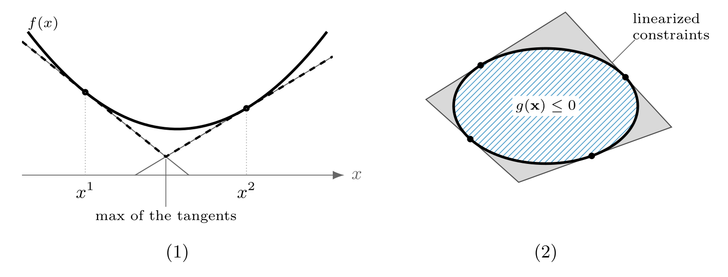
At each evaluated point , define and analogous row tangents . The accumulated master is
Convexity gives and componentwise. Every original feasible epigraph point therefore satisfies every tangent row. Global minimization of this relaxation gives a lower bound. The proof holds at any valid differentiability point, not only an optimal feasible one. For nonconvex , the tangent at excludes the original feasible point ; convexity cannot be silently dropped. Bonami et al. pp.188–191 gives the precise finite OA/KKT result.
Affine domain/coupling rows can be stored once. Each new point adds an objective tangent and the genuinely nonlinear constraint tangents. The insulation model below adds only one nonlinear objective row per iteration. Accumulating valid rows improves the master value for a fixed feasible-domain/exclusion convention, but does not itself remove a binary vector. Finite OA without explicit no-good cuts relies on the stated KKT/exactness and objective-improvement argument; the finite exclusion variant below is a different transparent teaching procedure.
Integer exclusions and the correct global certificate¶
For a visited binary vector , let and . The Hamming inequality
excludes exactly that vector and no other binary vector. Equivalently . This is an exclusion for the remaining search, not necessarily a valid inequality for the original feasible set. A previously evaluated optimum may be excluded because its value is retained separately. A local failure or an unevaluated design is not a justification for excluding it.
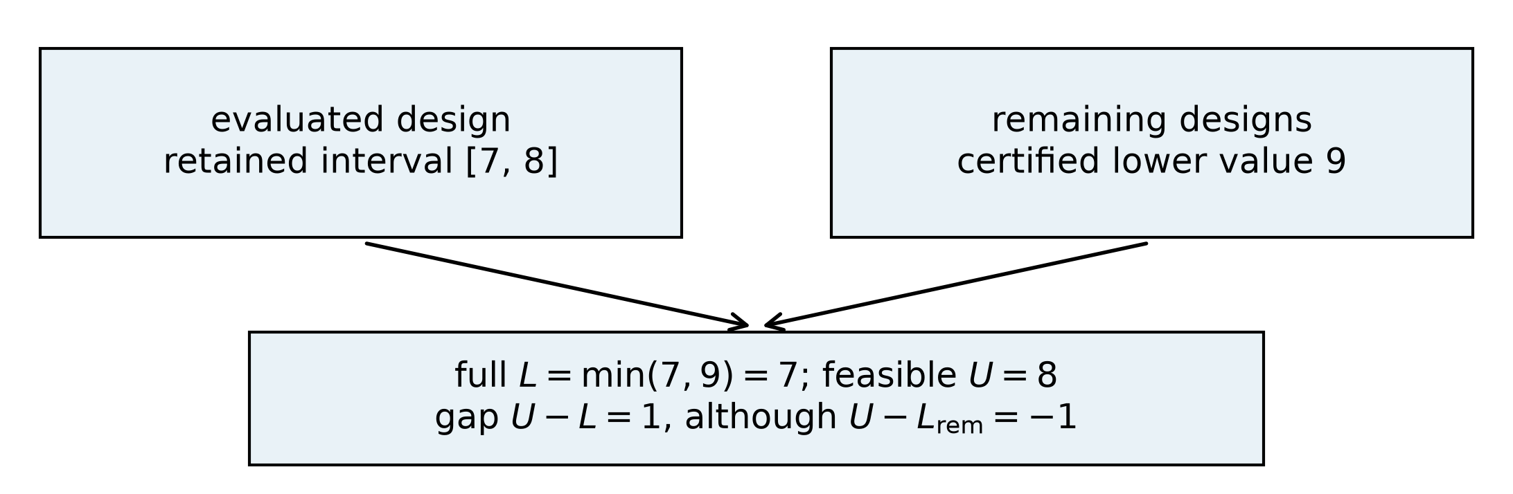
Let be the evaluated feasible designs, and let be the globally solved master value on all remaining designs. With exact evaluated values, and
Indeed, the original optimum is the smaller of the evaluated-design optimum and the remaining-design optimum; the master bounds only the latter. Thus may exceed after an optimal design is excluded. A negative raw difference means no remaining candidate can improve , not a negative global optimality gap.
For approximate evaluations, retain each certified design lower bound and feasible upper value . Then
Use for a tolerance certificate. Replacing the evaluated lower values by without proving their optimality can lose a better continuous solution of an excluded design. A valid infeasible master says no feasible remaining candidate; it need not mean every binary pattern was individually visited. With no incumbent, it proves original infeasibility only if all excluded designs were themselves certified infeasible.
A complete finite search and its failure statuses¶
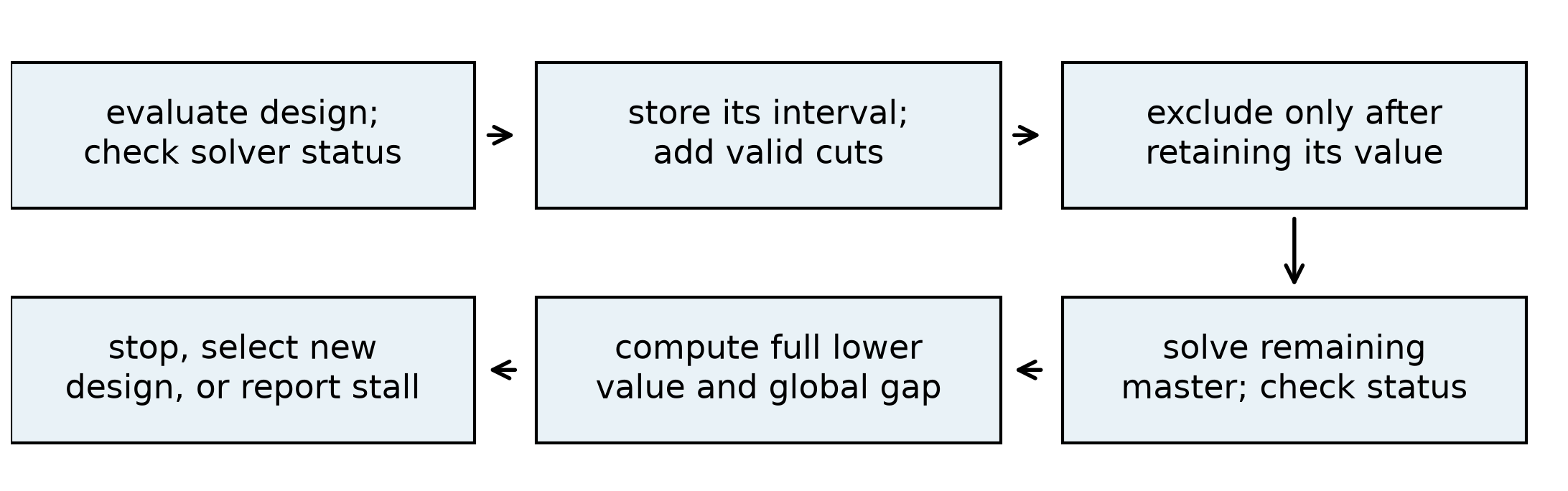
For the binary exclusion variant:
Choose a permitted binary vector, an initialized objective minorant, and explicit solver/gap/iteration limits.
Solve its continuous subproblem. Store an original-feasible upper value and a certified lower value. If infeasible, obtain a valid phase-I or other infeasibility certificate; do not equate solver failure with infeasibility.
Add objective/constraint tangents or valid GBD cuts. Add a no-good exclusion only after the evaluated value/certificate is retained.
Globally solve the remaining master. Handle infeasible, unbounded, interrupted and failed statuses before loading values. A valid infeasible master leaves only the evaluated-design bound calculation.
Form the full lower value above. Return convergence only when an incumbent exists and the requested global gap passes.
Otherwise choose the next unevaluated binary vector from the master. If the limiting uncertainty is a weak already-evaluated lower value, refine that design or report a certification stall. An iteration cap returns an incumbent with an explicit limit status.
With finite and exact/certified design decisions, no design is revisited and at most design evaluations are needed by this enumeration variant. This is a finite-search bound, not a claim that every NLP or MILP solve terminates successfully. In the affine limiting case, an exact master can settle the search in one evaluation when the start is already optimal, or after a second evaluation of its predicted optimum. BGW’s reported 3–5 iterations is a historical observation, not a universal rate guarantee.
The executable insulation search implements status-aware feasible-design evaluation and the full gap using retained lower values. Every binary design of this particular model is feasible at zero thickness. Its failure branch returns a solver-failure status; it does not implement a general phase-I/restoration solver. The reference above and the GBD feasibility argument below specify that general branch separately.
Insulation model, derivatives and independent validation¶
A layered wall has , with thicknesses , conductivity , and . Its illustrative annual cost is
The five materials and exact parameters are supplied in the executable table below; per-layer caps and the fifth material are course additions. The application/data are adapted from Postek, Zocca, Gromicho and Kantor, Hands-On Mathematical Optimization with Python, notebook 6.4. Its conic formulation is replaced here by OA/GBD. Retain the original source/licence notice with the adapted code: Copyright(c)2022 Jeffrey Kantor, MIT-licensed. The costs are teaching data, not quotations for constructing a wall.
Set . For the continuous objective ,
For every direction , . The Hessian is generally rank 1, not positive definite. The availability and thickness rows are affine, so every fixed-design problem is convex. Successful local minimization has the global convex interpretation, while numerical feasibility, residuals and termination still need checking.
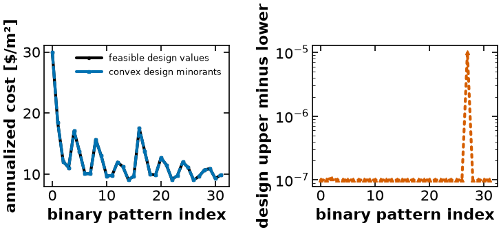
Independent optimization of all 32 binary designs, with feasible-point repair and linear-domain dual minorants, confirms the best pattern : fiberglass .04 m, mineral wool .06 m and high-R foam .05 m. Total thickness is .15 m, resistance , and annualized cost 9.0700 per square meter. The portable audit’s numerical global interval is approximately ; the code below performs its own model checks and shared algorithm runs. This is a numerical certificate supported by convexity/duality, not formal interval arithmetic. Bonmin independently solves the same model in the original comparison cell.
Generalized Benders cuts, domain normals and feasibility¶
Assume KKT holds at a convex fixed-design solution. For that solution and its nonnegative coupled multipliers , KKT with the normal cone of gives
Thus minimizes over . At any original feasible ,
The right side is an affine objective cut in alone. Complementarity makes it agree with the exact design objective at . Domain bounds/affine rows are part of ; do not demand unconstrained zero stationarity. A multiplier-derived affine minorant can be a subgradient support of a nondifferentiable value function, not necessarily its unique derivative. BGW pp.766–768; Grossmann pp.234–235.
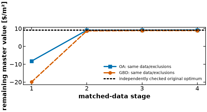
For the matched OA master, add the objective tangent and the constraint tangents weighted by . Their sum implies , where . Exact domain stationarity makes the last term nonnegative for every . Hence each GBD cut is implied by OA; projecting out can lose information. Identical points/domains/exclusions imply . Different adaptive runs are not theorem-ordered at the same iteration, and the proof alone does not order every runtime or iteration count.
For an infeasible phase-I optimum with value , its free-scalar KKT row gives , , and domain stationarity makes minimize over . Complementarity gives . Therefore the feasibility cut holds for every feasible design and excludes . This is not an objective cut. Residual-aware domain minimization can strengthen its validity checks too. Before any feasible objective cut exists, initialize a valid objective minorant; otherwise an unconstrained epigraph can leave the GBD master unbounded. Grossmann p.234 distinguishes feasible/infeasible subproblem cuts.
An explicit epigraph initialization chooses any differentiability point and sets . The valid initial objective row is . Compact polyhedral makes this linear minimization finite. This row does not require a previously feasible coupled design. For an approximate phase-I multiplier vector, the analogous weighted constraint tangent plus its domain minimum is a valid feasibility minorant; a positive value at the candidate design must be certified before that cut is used to exclude it.
Approximate multipliers: a valid domain correction¶
For an approximate point and any nonnegative candidate , let and
Convex tangents and the nonnegative weighted feasibility rows imply the corrected objective minorant
It does not assume exact KKT stationarity. For insulation , linear minimization is attained at 0 or , so . The same corrected expression at a fixed design bounds its continuous optimum, allowing it to be retained when that binary pattern is excluded.
Without correction, , , coupling , approximate and would give the false constant bound .25 at , whose true value is 0. Here , and the corrected bound is . At an exact domain-stationary point the correction is 0, recovering the usual formula.
The original insulation first solve has complementarity sum : its raw cut exceeds the reported relaxed NLP value by that amount. Against independently solved original designs, its largest observed overrun is only , not 10-5. A domain correction places it below all 32 checked values. A zero complementarity product would remain zero after reversing the multiplier sign, so agreement at one point cannot test signs; check nonnegativity, domain stationarity/correction and other designs.
When imported duals produce a weak minorant, the revised search also fits nonnegative KKT candidates on the active availability, lower-bound and total-thickness rows at a repaired feasible point. It chooses the stronger of the two corrected design lower values. The domain correction remains necessary; fitting does not establish exact stationarity.
The revised search imports upper-row duals with the sign reversed, projects tiny negative candidates to nonnegative values, repairs a returned primal point into the original thickness/cap domain, and computes a domain minorant from the raw point and candidate duals. It reports a small explicit numerical guard on that lower value and retains both design/global gaps. These guards are numerical safeguards; do not describe floating-point outputs as formal interval proofs.
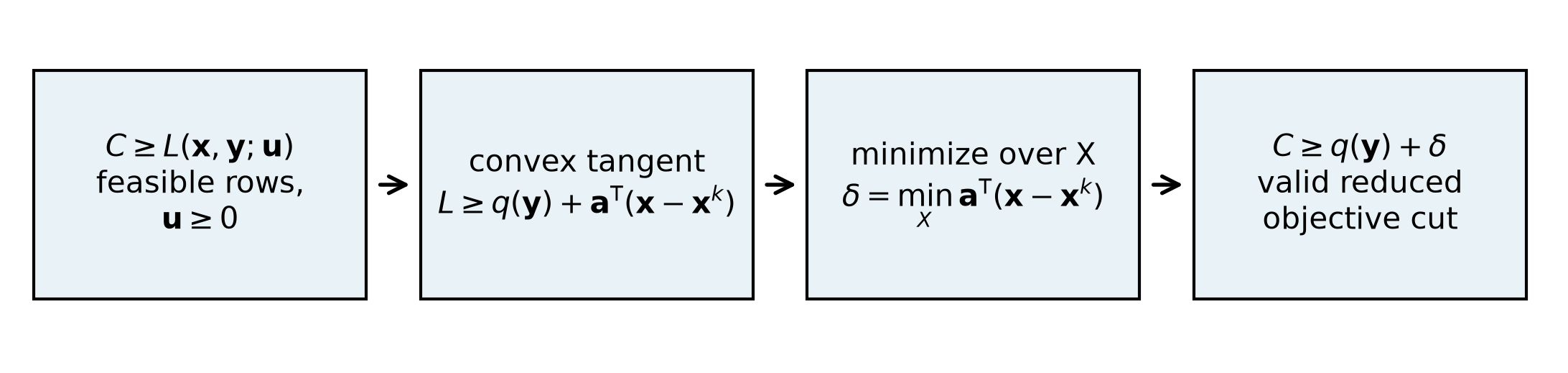
Here C is the original objective, L its Lagrangian, and q the affine cut expression before the domain correction.
Controlled comparisons, tools and sources¶
The original demonstration takes three OA and four GBD major iterations; BGW’s separate example has the same counts. These are observations on different models. The matched experiment below instead supplies identical points and exclusions to both masters, testing the surrogate inequality directly. In the insulation model OA adds one objective row per point plus stored affine/domain constraints; GBD adds one corrected objective cut and eliminates . Its smaller master can lose useful domain information even though row growth here is the same.
Bonmin implements convex MINLP algorithms; its nonconvex use is heuristic. DICOPT uses OA/equality-relaxation/penalty variants through GAMS and does not promise a nonconvex global optimum. Pyomo supplies a GAMS interface. MindtPy provides decomposition strategies and documented solver/tolerance options. Check installed support, termination and bounds when choosing those options. Assignment Algorithms 6 uses MindtPy; this reference supplies the mechanisms without transferring graded solutions.
Primary reading: BGW Appendix A §A.3.2 pp.757–761 and §A.3.4 pp.763–768; Bonami et al., An algorithmic framework for convex mixed integer nonlinear programs, pp.187–191; Grossmann, Review of nonlinear mixed-integer and disjunctive programming techniques, pp.234–235. Duran–Grossmann supplies the original OA formulation, Geoffrion the generalized Benders framework, and Quesada–Grossmann the LP/NLP branch-and-bound relationship. General modeling, stochastic-programming and convexity recaps retain their existing canonical reference homes.
Executable setup¶
# This code cell installs packages on Colab

import sys

if "google.colab" in sys.modules:
    !wget "https://raw.githubusercontent.com/ndcbe/optimization/main/notebooks/helper.py"
    import helper

    helper.easy_install()
else:
    sys.path.insert(0, "../")
    import helper

helper.set_plotting_style()
import numpy as np
import pandas as pd
import matplotlib.pyplot as plt
import pyomo.environ as pyo
# House figure style. On Colab only the notebook is present, so fall back to the raw URL.
STYLE = (
"https://raw.githubusercontent.com/ndcbe/optimization/main/figures/dowling.mplstyle"
if "google.colab" in sys.modules
else "../../figures/dowling.mplstyle"
)
plt.style.use(STYLE)
solver_milp = pyo.SolverFactory("appsi_highs")
solver_nlp = pyo.SolverFactory("ipopt")Branch and bound: actual LP models and search¶
Node status is checked before values are loaded. This example is bounded below; ambiguous termination is reported as failure. Rounded integer candidates are checked in the original covering row.
def build_mipex_relaxation(fixed=None):
    """LP relaxation of (MIPEX) with some binaries fixed.

    Arguments:
        fixed: dict mapping binary index (1, 2, 3) to the value it is fixed at

    Returns:
        a Pyomo ConcreteModel
    """
    m = pyo.ConcreteModel("MIPEX LP relaxation")
    m.J = pyo.RangeSet(1, 3)

    m.x = pyo.Var(domain=pyo.NonNegativeReals)
    m.y = pyo.Var(m.J, bounds=(0, 1))  # integrality relaxed to the unit box

    @m.Constraint()
    def coupling(m):
        """Link the continuous variable to the binary decisions."""
        return -m.x + 3 * m.y[1] + 2 * m.y[2] + m.y[3] <= 0

    @m.Constraint()
    def covering(m):
        """Enforce the minimum binary coverage requirement."""
        return -5 * m.y[1] - 8 * m.y[2] - 3 * m.y[3] <= -9

    @m.Objective(sense=pyo.minimize)
    def z(m):
        """Minimize the relaxation objective."""
        return m.x + m.y[1] + 3 * m.y[2] + 2 * m.y[3]

    for j, value in (fixed or {}).items():
        m.y[j].fix(value)

    return m


def solve_node(fixed):
    """Solve one node's LP relaxation and report what happened.

    An infeasible relaxation is an ANSWER here, not a failure -- it fathoms a whole
    subtree. So the termination condition is checked explicitly and `load_solutions`
    is deferred: HiGHS raises if asked to load a solution that does not exist.
    """
    m = build_mipex_relaxation(fixed)
    results = solver_milp.solve(m, load_solutions=False)
    tc = results.solver.termination_condition

    if pyo.check_optimal_termination(results):
        m.solutions.load_from(results)
        return {
            "status": "optimal",
            "z": pyo.value(m.z),
            "y": np.array([pyo.value(m.y[j]) for j in m.J]),
            "x": pyo.value(m.x),
        }
    if tc == pyo.TerminationCondition.infeasible:
        return {"status": "infeasible", "z": None, "y": None, "x": None}

    raise RuntimeError(f"unexpected termination condition at node {fixed}: {tc}")
INT_TOL = 1e-6
GAP_TOL = 1e-9
def branch_and_bound(verbose=True):
"""Breadth-first branch and bound on (MIPEX).
Returns:
nodes: list of dicts, one per node, in the order the LPs were solved
edges: list of (parent, child, label) tuples describing the tree
incumbent: dict with the optimal solution
"""
incumbent_z, incumbent = np.inf, None
queue = [{"fixed": {}, "parent": None, "label": ""}] # FIFO -> breadth first
nodes, edges = [], []
node_id = 0
while queue:
node = queue.pop(0)
node_id += 1
result = solve_node(node["fixed"])
if node["parent"] is not None:
edges.append((node["parent"], node_id, node["label"]))
record = {
"node": node_id,
"fixed": ", ".join(f"y{j}={v}" for j, v in node["fixed"].items()) or "--",
"z_LP": result["z"],
"y_LP": None if result["y"] is None else np.round(result["y"], 4),
}
# case 1a: the relaxation has no feasible point, so neither does the subtree
if result["status"] == "infeasible":
record.update(case=1, outcome="infeasible -> fathom")
# case 1b: the bound is already worse than a solution we hold in hand
elif result["z"] >= incumbent_z - GAP_TOL:
record.update(
case=1, outcome=f"bound {result['z']:.2f} >= incumbent -> fathom"
)
else:
fractional = [
j
for j in (1, 2, 3)
if abs(result["y"][j - 1] - round(result["y"][j - 1])) > INT_TOL
]
# case 2: the relaxation happened to land on an integer point
if not fractional:
rounded = np.round(result["y"]).astype(int)
if np.dot([5, 8, 3], rounded) < 9:
raise RuntimeError("Rounded LP candidate violates the original covering row.")
checked_x = float(np.dot([3, 2, 1], rounded))
checked_z = checked_x + float(np.dot([1, 3, 2], rounded))
if checked_z - result["z"] > GAP_TOL:
raise RuntimeError("Integer-candidate gap needs refinement before closing this node.")
incumbent_z, incumbent = checked_z, {**result, "y": rounded, "x": checked_x, "z": checked_z, "node": node_id}
record.update(
case=2, outcome=f"integral -> incumbent z = {result['z']:.0f}"
)
# case 3: branch
else:
j = fractional[0]
record.update(case=3, outcome=f"branch on y{j}")
for value in (0, 1):
queue.append(
{
"fixed": {**node["fixed"], j: value},
"parent": node_id,
"label": f"$y_{j}$={value}",
}
)
nodes.append(record)
if verbose:
z_text = (
"infeasible" if record["z_LP"] is None else f"{record['z_LP']:8.4f}"
)
print(
f"node {node_id}: fixed {record['fixed']:<20s} z_LP = {z_text} {record['outcome']}"
)
return nodes, edges, incumbent
nodes, edges, incumbent = branch_and_bound()node 1: fixed -- z_LP = 5.8000 branch on y1
node 2: fixed y1=0 z_LP = 6.0000 branch on y3
node 3: fixed y1=1 z_LP = 6.5000 branch on y2
node 4: fixed y1=0, y3=0 z_LP = infeasible infeasible -> fathom
node 5: fixed y1=0, y3=1 z_LP = 6.7500 branch on y2
node 6: fixed y1=1, y2=0 z_LP = infeasible infeasible -> fathom
node 7: fixed y1=1, y2=1 z_LP = 9.0000 integral -> incumbent z = 9
node 8: fixed y1=0, y3=1, y2=0 z_LP = infeasible infeasible -> fathom
node 9: fixed y1=0, y3=1, y2=1 z_LP = 8.0000 integral -> incumbent z = 8
bb_data = {"nodes": nodes, "edges": edges, "incumbent": incumbent}
results = bb_data
helper.save_results("minlp-search-actual", bb_data, notebook="notebooks/8-dev/MINLP-Algorithms.ipynb",
 source_cells=[("notebooks/8-dev/MINLP-Algorithms.ipynb", "results:minlp-original-02"), ("notebooks/8-dev/MINLP-Algorithms.ipynb", "results:minlp-original-04"), ("notebooks/8-dev/MINLP-Algorithms.ipynb", "results:minlp-original-06")],
 description="Actual Pyomo/HiGHS breadth-first search and checked integer candidates", solver="appsi_highs", quiet=True)
table = pd.DataFrame(nodes).set_index("node")
display(table)

print(f"\nz*  = {incumbent['z']:.0f}")
print(f"y*  = {np.round(incumbent['y']).astype(int)}")
print(f"x*  = {incumbent['x']:.0f}   (found at node {incumbent['node']})")
print(f"\n{len(nodes)} nodes examined out of the 15 in the full tree")
z*  = 8
y*  = [0 1 1]
x*  = 3   (found at node 9)

9 nodes examined out of the 15 in the full tree
def plot_tree(nodes, edges, ax=None):
    """Draw the branch and bound tree from the node records and edge list."""
    table = {n["node"]: n for n in nodes}

    depth = {1: 0}
    children = {}
    for parent, child, _ in edges:
        depth[child] = depth[parent] + 1
        children.setdefault(parent, []).append(child)

    # tidy layout: leaves get consecutive slots left to right, a parent sits
    # at the midpoint of its children
    x_of = {}
    next_slot = [0.0]

    def place(node_id):
        """Assign horizontal positions recursively to tree nodes."""
        kids = children.get(node_id, [])
        if not kids:
            x_of[node_id] = next_slot[0]
            next_slot[0] += 1.0
        else:
            for kid in kids:
                place(kid)
            x_of[node_id] = 0.5 * (x_of[kids[0]] + x_of[kids[-1]])

    place(1)
    pos = {node_id: (x_of[node_id], -depth[node_id]) for node_id in depth}

    if ax is None:
        _, ax = plt.subplots(figsize=(7.5, 4.5))

    for parent, child, label in edges:
        (x0, y0), (x1, y1) = pos[parent], pos[child]
        ax.plot([x0, x1], [y0, y1], color="0.45", lw=1.5, ls="-", zorder=1)
        ax.annotate(
            label,
            xy=(x0 + 0.62 * (x1 - x0), y0 + 0.62 * (y1 - y0)),
            ha="center",
            va="center",
            fontsize=11,
            bbox=dict(boxstyle="round,pad=0.12", fc="white", ec="none"),
            zorder=2,
        )

    for node_id, (x, y) in pos.items():
        record = table[node_id]
        # case 2 nodes (integer solutions) are filled; everything else is open
        filled = record["case"] == 2
        ax.plot(
            x,
            y,
            marker="o",
            ms=26,
            mfc="black" if filled else "white",
            mec="black",
            mew=1.8,
            zorder=3,
        )
        ax.annotate(
            str(node_id),
            xy=(x, y),
            ha="center",
            va="center",
            fontsize=13,
            color="white" if filled else "black",
            zorder=4,
        )
        text = "infeas." if record["z_LP"] is None else f"$z={record['z_LP']:g}$"
        ax.annotate(
            text, xy=(x + 0.20, y), ha="left", va="center", fontsize=12, zorder=4
        )

    ax.set_xlim(min(x_of.values()) - 0.6, max(x_of.values()) + 0.9)
    ax.set_ylim(-max(depth.values()) - 0.5, 0.5)
    ax.axis("off")
    return ax


fig, ax = plt.subplots(figsize=(7.6, 3.5))
plot_tree(results["nodes"], results["edges"], ax=ax)
ax.set_title(
    "Branch and bound tree, breadth first\n(filled = integer solution)", fontsize=14
)
fig.tight_layout()
helper.save_figure(fig, "minlp-search-actual", quiet=True)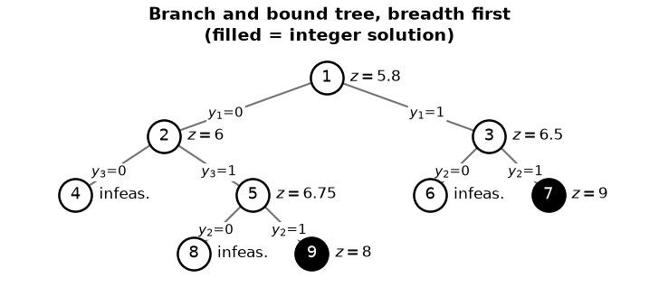
Independent MILP comparison¶
def build_mipex_milp():
    """(MIPEX) with the integrality restored."""
    m = build_mipex_relaxation()
    for j in m.J:
        m.y[j].domain = pyo.Binary
    return m


m = build_mipex_milp()
results = solver_milp.solve(m, load_solutions=False)
assert pyo.check_optimal_termination(
    results
), f"MILP solve failed: {results.solver.termination_condition}"
m.solutions.load_from(results)

print(
    f"HiGHS: z* = {pyo.value(m.z):.0f}, "
    f"y* = {[round(pyo.value(m.y[j])) for j in m.J]}, x* = {pyo.value(m.x):.0f}"
)
assert (
    abs(pyo.value(m.z) - incumbent["z"]) < 1e-6
), "our branch and bound disagrees with HiGHS"
HiGHS: z* = 8, y* = [0, 1, 1], x* = 3
Insulation: exact teaching data and model¶
The application is adapted as described above; the original Copyright (c) 2022 Jeffrey Kantor/MIT source notice is retained. Per-layer caps and the fifth material are course additions.
# k: thermal conductivity [W/m/K]; a: fixed installation cost [$/m^2];
# b: installed material cost [$/m^3]; tmax: largest available thickness [m]
materials = pd.DataFrame(
    {
        "Fiberglass batt": {"k": 0.040, "a": 4.0, "b": 60.0, "tmax": 0.06},
        "Mineral wool": {"k": 0.030, "a": 5.0, "b": 150.0, "tmax": 0.06},
        "Rigid foam (low R)": {"k": 0.030, "a": 8.0, "b": 120.0, "tmax": 0.05},
        "Rigid foam (high R)": {"k": 0.015, "a": 8.0, "b": 180.0, "tmax": 0.05},
        "Aerogel blanket": {"k": 0.013, "a": 12.0, "b": 900.0, "tmax": 0.02},
    }
).T

ALPHA = 60.0  # annualized energy cost per unit U   [$ K / W / yr]
BETA = 0.05  # equivalent annual cost factor on capital [1/yr]
R0 = 2.0  # resistance of the structural elements  [m^2 K / W]
T_TOTAL = 0.15  # total thickness the wall cavity allows [m]

display(materials)economics = pd.DataFrame(
{
"capital cost per R [$ W / (m^4 K)]": materials["b"] * materials["k"],
"R per thickness [m K/W]": 1.0 / materials["k"],
"fixed charge [$/m^2/yr]": BETA * materials["a"],
}
)
display(economics.round(2))def thermal_resistance(x):
"""R = R0 + sum_n x_n / k_n for a dict of thicknesses."""
return R0 + sum(x[n] / materials.loc[n, "k"] for n in materials.index)
def f_continuous(x):
"""The nonlinear part of the objective, f(x): energy cost plus material cost."""
return ALPHA / thermal_resistance(x) + BETA * sum(
materials.loc[n, "b"] * x[n] for n in materials.index
)
def grad_f_continuous(x):
"""Gradient of f at x. d/dx_n [alpha / R] = -alpha / R^2 / k_n."""
R = thermal_resistance(x)
return {
n: -ALPHA / R**2 / materials.loc[n, "k"] + BETA * materials.loc[n, "b"]
for n in materials.index
}Continuous restrictions and original-model feasibility¶
def build_nlp_subproblem(y):
    """NLP subproblem of outer approximation: the design cost with the layers y fixed.

    Arguments:
        y: dict mapping material name to 0 or 1

    Returns:
        a Pyomo ConcreteModel
    """
    m = pyo.ConcreteModel("insulation NLP subproblem")
    m.N = pyo.Set(initialize=list(materials.index))
    m.x = pyo.Var(m.N, domain=pyo.NonNegativeReals, bounds=(0, T_TOTAL))

    @m.Constraint(m.N)
    def layer_available(m, n):
        """Allow thickness only when material n is selected."""
        return m.x[n] <= materials.loc[n, "tmax"] * y[n]

    @m.Constraint()
    def thickness_budget(m):
        """Limit the total insulation thickness."""
        return sum(m.x[n] for n in m.N) <= T_TOTAL

    @m.Objective(sense=pyo.minimize)
    def cost(m):
        """Minimize annualized heat-loss and material costs."""
        R = R0 + sum(m.x[n] / materials.loc[n, "k"] for n in m.N)
        return (
            ALPHA / R
            + BETA * sum(materials.loc[n, "b"] * m.x[n] for n in m.N)
            + BETA
            * sum(materials.loc[n, "a"] * y[n] for n in m.N)  # c^T y, a constant here
        )

    return m


def solve_nlp_subproblem(y):
    """Solve the NLP subproblem and return (x^k, z^u)."""
    m = build_nlp_subproblem(y)
    results = solver_nlp.solve(m)
    assert pyo.check_optimal_termination(
        results
    ), f"NLP subproblem failed for y = {y}: {results.solver.termination_condition}"
    return {n: pyo.value(m.x[n]) for n in materials.index}, pyo.value(m.cost)
OA remaining-design master¶
Affine coupling rows are stored once; objective tangents accumulate. Integer exclusions change the designs being bounded.
def build_master_problem(points, tried):
    """MILP master problem of outer approximation.

    Arguments:
        points: list of x^k dicts, one per iteration so far -- the linearization points
        tried:  list of y^k dicts already evaluated, each excluded by an integer cut

    Returns:
        a Pyomo ConcreteModel
    """
    m = pyo.ConcreteModel("outer approximation master MILP")
    m.N = pyo.Set(initialize=list(materials.index))
    m.x = pyo.Var(m.N, domain=pyo.NonNegativeReals, bounds=(0, T_TOTAL))
    m.y = pyo.Var(m.N, domain=pyo.Binary)
    m.epi = pyo.Var(domain=pyo.Reals)  # the epigraph variable, zeta in the reference

    @m.Constraint(m.N)
    def layer_available(m, n):
        """Allow thickness only when material n is selected."""
        return m.x[n] <= materials.loc[n, "tmax"] * m.y[n]

    @m.Constraint()
    def thickness_budget(m):
        """Limit the total insulation thickness."""
        return sum(m.x[n] for n in m.N) <= T_TOTAL

    # one outer approximation of the objective per point visited: since f is convex,
    # every tangent plane lies below f, so each row is a valid relaxation
    m.outer_approximation = pyo.ConstraintList()
    for xk in points:
        fk = f_continuous(xk)
        gk = grad_f_continuous(xk)
        m.outer_approximation.add(
            m.epi
            >= BETA * sum(materials.loc[n, "a"] * m.y[n] for n in m.N)
            + fk
            + sum(gk[n] * (m.x[n] - xk[n]) for n in m.N)
        )

    # integer cuts: at least one component of y must differ from each y^k already tried
    m.integer_cuts = pyo.ConstraintList()
    for yk in tried:
        ones = [n for n in m.N if yk[n] > 0.5]
        zeros = [n for n in m.N if yk[n] <= 0.5]
        m.integer_cuts.add(
            sum(m.y[n] for n in ones) - sum(m.y[n] for n in zeros) <= len(ones) - 1
        )

    @m.Objective(sense=pyo.minimize)
    def lower_bound(m):
        """Minimize the master-problem epigraph bound."""
        return m.epi

    return m
Status-aware OA search¶
from scipy.optimize import nnls

def domain_correction(xk, uk):
    """Minimize the Lagrangian tangent over the common thickness simplex X."""
    slope = {n: grad_f_continuous(xk)[n] + max(0.0, uk[n]) for n in materials.index}
    return T_TOTAL * min(0.0, min(slope.values())) - sum(slope[n] * xk[n] for n in materials.index)


def benders_guard(xk, uk):
    """Return the explicitly scaled numerical guard used on affine minorants."""
    intercept = f_continuous(xk) + sum(max(0.0, uk[n]) * xk[n] for n in materials.index) + domain_correction(xk, uk)
    return 1e-8 * (1 + abs(intercept) + sum(abs(max(0.0, uk[n]) * materials.loc[n, "tmax"]) for n in materials.index))


def evaluate_design(y, fit_multipliers=True):
    """Return a feasible original-domain upper value and a convex dual minorant."""
    if set(y) != set(materials.index) or any(value not in (0, 1) for value in y.values()):
        raise ValueError("A binary value is required for every material.")
    model = build_nlp_subproblem(y)
    model.dual = pyo.Suffix(direction=pyo.Suffix.IMPORT)
    result = solver_nlp.solve(model, options={"tol": 1e-9, "bound_relax_factor": 0})
    if not pyo.check_optimal_termination(result):
        raise RuntimeError(f"Fixed-design solve failed: {result.solver.termination_condition}")
    raw = {n: pyo.value(model.x[n]) for n in materials.index}
    u = {n: max(0.0, -model.dual[model.layer_available[n]]) for n in materials.index}
    # The repaired point is feasible in the original domain; it supplies U.
    x = {n: min(max(raw[n], 0.0), materials.loc[n, "tmax"] * y[n]) for n in materials.index}
    total = sum(x.values())
    if total > T_TOTAL:
        x = {n: value * T_TOTAL / total for n, value in x.items()}
    fixed = BETA * sum(materials.loc[n, "a"] * y[n] for n in materials.index)
    upper = fixed + f_continuous(x)
    # Degenerate zero-availability rows can give large imported duals. Fit a
    # second nonnegative candidate at the repaired point, retaining the domain
    # correction: a small stationarity residual is not assumed to be zero.
    names = list(materials.index)
    cap = np.array([materials.loc[n, "tmax"] * y[n] for n in names])
    point = np.array([x[n] for n in names])
    active = np.r_[cap - point <= 1e-7, point <= 1e-7, T_TOTAL - point.sum() <= 1e-7]
    columns = np.c_[np.eye(len(names)), -np.eye(len(names)), np.ones(len(names))]
    coefficients = np.zeros(2 * len(names) + 1)
    coefficients[active], fit_residual = nnls(columns[:, active], -np.array([grad_f_continuous(x)[n] for n in names]))
    fitted_u = {n: float(coefficients[i]) for i, n in enumerate(names)}
    candidates = []
    for cut_x, candidate_u, origin in [(raw, u, "imported"), (x, fitted_u, "fitted")]:
        correction = domain_correction(cut_x, candidate_u)
        intercept = f_continuous(cut_x) + sum(candidate_u[n] * cut_x[n] for n in names) + correction
        guard = benders_guard(cut_x, candidate_u)
        lower = fixed + intercept - sum(candidate_u[n] * materials.loc[n, "tmax"] * y[n] for n in names) - guard
        candidates.append({"lower": lower, "cut_x": cut_x, "u": candidate_u, "domain_correction": correction,
                           "numerical_guard": guard, "multiplier_origin": origin})
    chosen = max(candidates, key=lambda candidate: candidate["lower"]) if fit_multipliers else candidates[0]
    if chosen["lower"] > upper + 1e-7:
        raise RuntimeError("Design minorant exceeds its feasible upper value.")
    violation = max(0.0, sum(x.values()) - T_TOTAL, max(x[n] - materials.loc[n, "tmax"] * y[n] for n in names), max(-value for value in x.values()))
    return {"y": dict(y), "raw_x": raw, "x": x, "upper": upper, **chosen,
            "imported_u": u, "candidate_lowers": {item["multiplier_origin"]: item["lower"] for item in candidates},
            "fitted_stationarity_residual": float(fit_residual), "original_violation": violation,
            "reported_NLP_objective": pyo.value(model.cost)}


def decomposition_search(y_start, strategy="OA", eps=1e-4, max_iter=20, verbose=True, fit_multipliers=True):
    """Search feasible insulation designs while retaining their lower/upper values."""
    if strategy not in ("OA", "GBD") or max_iter < 1 or eps <= 0:
        raise ValueError("Use OA or GBD, a positive gap tolerance, and at least one iteration.")
    y = dict(y_start)
    points, cuts, tried, evaluations, rows = [], [], [], [], []
    upper, best, status = np.inf, None, "iteration_limit"
    remaining, global_lower = -np.inf, -np.inf
    for iteration in range(1, max_iter + 1):
        if any(y == old for old in tried):
            status = "repeated_design"
            break
        try:
            evaluated = evaluate_design(y, fit_multipliers=fit_multipliers)
        except RuntimeError as error:
            status = "solver_failure"
            failure = str(error)
            break
        evaluations.append(evaluated)
        points.append(evaluated["cut_x"])
        cuts.append((evaluated["cut_x"], evaluated["u"]))
        tried.append(dict(y))
        if evaluated["upper"] < upper:
            upper, best = evaluated["upper"], (dict(y), dict(evaluated["x"]))
        master = build_master_problem(points, tried) if strategy == "OA" else build_gbd_master(cuts, tried)
        solved = solver_milp.solve(master, load_solutions=False, options={"mip_rel_gap": 0})
        tc = solved.solver.termination_condition
        exhausted = tc == pyo.TerminationCondition.infeasible
        if exhausted:
            remaining = np.inf
        elif pyo.check_optimal_termination(solved):
            master.solutions.load_from(solved)
            remaining = float(solved.problem.lower_bound)
            if not np.isfinite(remaining):
                status = "missing_master_bound"
                break
        else:
            status = "master_failure"
            failure = str(tc)
            break
        # Previously evaluated designs remain in the original optimization problem.
        evaluated_lower = min(item["lower"] for item in evaluations)
        global_lower = min(remaining, evaluated_lower)
        gap = upper - global_lower
        rows.append({"iteration": iteration, "z_nlp": evaluated["reported_NLP_objective"],
                     "z_upper": upper, "z_lower": remaining, "z_global_lower": global_lower,
                     "global_gap": gap, "design_lower": evaluated["lower"],
                     "original_violation": evaluated["original_violation"], "layers": sum(y.values())})
        if verbose:
            print(f"{strategy} iteration {iteration}: U={upper:.6f}, remaining={remaining:.6f}, "
                  f"global L={global_lower:.6f}, gap={gap:.3e}")
        if gap <= eps:
            status = "converged"
            break
        if exhausted or remaining >= upper:
            status = "evaluated_design_gap"
            break
        y = {n: int(round(pyo.value(master.y[n]))) for n in materials.index}
    history = pd.DataFrame(rows)
    if not history.empty:
        history = history.set_index("iteration")
    history.attrs.update(status=status, strategy=strategy, global_lower=global_lower,
                         remaining_lower=remaining, upper=upper, evaluations=evaluations,
                         failure=locals().get("failure"), requested_gap=eps)
    if verbose:
        print(f"{strategy} status: {status}; feasible incumbent={upper:.6f}")
    return history, best, upper
def outer_approximation(y_start, eps=1e-4, max_iter=20, verbose=True):
    """Return the status-aware OA history, feasible incumbent and its upper value."""
    return decomposition_search(y_start, "OA", eps, max_iter, verbose)


y_start = {n: (1 if n == "Aerogel blanket" else 0) for n in materials.index}
history, best, oa_cost = outer_approximation(y_start)
assert history.attrs["status"] == "converged"
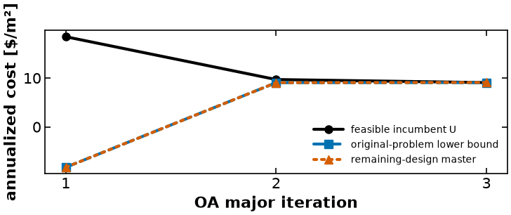
OA iteration 1: U=18.456522, remaining=-8.270841, global L=-8.270841, gap=2.673e+01
OA iteration 2: U=9.698077, remaining=9.059349, global L=9.059349, gap=6.387e-01
OA iteration 3: U=9.070000, remaining=9.098077, global L=9.070000, gap=1.311e-07
OA status: converged; feasible incumbent=9.070000
oa_data = {"history": history.reset_index().to_dict("records"), "status": history.attrs["status"],
 "best_y": best[0], "best_x": best[1], "upper": oa_cost, "global_lower": history.attrs["global_lower"]}
results = oa_data
helper.save_results("minlp-oa-actual", oa_data, notebook="notebooks/8-dev/MINLP-Algorithms.ipynb",
 source_cells=[("notebooks/8-dev/MINLP-Algorithms.ipynb", "results:" + name) for name in ["minlp-original-02", "minlp-original-15", "minlp-original-18", "minlp-original-20", "minlp-original-22", "minlp-controller", "minlp-original-24"]],
 description="Original and remaining bounds from the status-aware OA search", solver="ipopt and appsi_highs", quiet=True)
display(history.round(4))

y_best, x_best = best
solution = materials.copy()
solution["installed"] = [int(y_best[n]) for n in materials.index]
solution["x opt [m]"] = [max(x_best[n], 0.0) for n in materials.index]
display(solution[["k", "a", "b", "tmax", "installed", "x opt [m]"]].round(5))

print(f"optimal annualized cost = {oa_cost:0.4f} $/m^2")
print(
    f"total thickness         = {sum(max(v, 0.0) for v in x_best.values()):0.4f} m "
    f"(budget {T_TOTAL} m)"
)
print(f"overall resistance R = {thermal_resistance(x_best):0.3f} m^2 K / W")optimal annualized cost = 9.0700 $/m^2
total thickness = 0.1500 m (budget 0.15 m)
overall resistance R = 8.333 m^2 K / W
rows = results["history"]
k = [r["iteration"] for r in rows]
fig, ax = plt.subplots(figsize=(7.6, 3.0))
ax.plot(k, [r["z_upper"] for r in rows], color="black", marker="o", label="feasible incumbent U")
ax.plot(k, [r["z_global_lower"] for r in rows], color="#0072B2", marker="s", linestyle="--", label="original-problem lower bound")
ax.plot(k, [r["z_lower"] for r in rows], color="#D55E00", marker="^", linestyle=":", label="remaining-design master")
ax.set(xlabel="OA major iteration", ylabel="annualized cost [$/m²]", xticks=k)
ax.legend(fontsize=10); fig.tight_layout()
helper.save_figure(fig, "minlp-oa-actual", quiet=True)
Independent Bonmin comparison¶
def build_insulation_minlp():
    """The full MINLP, for a solver that can take it whole."""
    m = pyo.ConcreteModel("insulation MINLP")
    m.N = pyo.Set(initialize=list(materials.index))
    m.x = pyo.Var(m.N, domain=pyo.NonNegativeReals, bounds=(0, T_TOTAL))
    m.y = pyo.Var(m.N, domain=pyo.Binary)

    @m.Constraint(m.N)
    def layer_available(m, n):
        """Allow thickness only when material n is selected."""
        return m.x[n] <= materials.loc[n, "tmax"] * m.y[n]

    @m.Constraint()
    def thickness_budget(m):
        """Limit the total insulation thickness."""
        return sum(m.x[n] for n in m.N) <= T_TOTAL

    @m.Objective(sense=pyo.minimize)
    def cost(m):
        """Minimize annualized heat-loss and material costs."""
        R = R0 + sum(m.x[n] / materials.loc[n, "k"] for n in m.N)
        return ALPHA / R + BETA * sum(
            materials.loc[n, "a"] * m.y[n] + materials.loc[n, "b"] * m.x[n] for n in m.N
        )

    return m


m_minlp = build_insulation_minlp()
results = pyo.SolverFactory("bonmin").solve(m_minlp)
assert pyo.check_optimal_termination(
    results
), f"bonmin failed: {results.solver.termination_condition}"

print(f"bonmin: cost = {pyo.value(m_minlp.cost):0.4f} $/m^2")
print("        layers = " f"{[n for n in m_minlp.N if pyo.value(m_minlp.y[n]) > 0.5]}")
assert (
    abs(pyo.value(m_minlp.cost) - oa_cost) < 1e-3
), "our outer approximation disagrees with bonmin"
bonmin: cost = 9.0700 $/m^2
layers = ['Fiberglass batt', 'Mineral wool', 'Rigid foam (high R)']
GBD: dual import, domain correction and search¶
This first raw solve retains the original default settings to display its complementarity discrepancy. Agreement at one point does not test the multiplier sign. The following search uses original-domain primal repair and retained design minorants.
def solve_nlp_subproblem_with_duals(y):
    """Solve the OA/GBD NLP subproblem and also return the multipliers of the coupled rows.

    Arguments:
        y: dict mapping material name to 0 or 1

    Returns:
        (x^k, z^u, u^k) -- thicknesses, objective, and the non-negative multipliers of
        the availability constraints x_n <= tmax_n y_n
    """
    m = build_nlp_subproblem(y)
    m.dual = pyo.Suffix(direction=pyo.Suffix.IMPORT)

    results = solver_nlp.solve(m)
    assert pyo.check_optimal_termination(
        results
    ), f"NLP subproblem failed for y = {y}: {results.solver.termination_condition}"

    xk = {n: pyo.value(m.x[n]) for n in materials.index}
    # Pyomo/Ipopt hands back non-positive duals for "<=" rows in a minimization;
    # the handout's u^k is non-negative, so flip the sign.
    uk = {n: -m.dual[m.layer_available[n]] for n in materials.index}
    return xk, pyo.value(m.cost), uk
xk0, zk0, uk0 = solve_nlp_subproblem_with_duals(y_start)
print("multipliers u^1 (all should be >= 0):")
for n in materials.index:
print(f" {n:22s} {uk0[n]:10.3f}")
complementarity = sum(
uk0[n] * (xk0[n] - materials.loc[n, "tmax"] * y_start[n]) for n in materials.index
)
cut_at_yk = (
BETA * sum(materials.loc[n, "a"] * y_start[n] for n in materials.index)
+ f_continuous(xk0)
+ complementarity
)
print(
f"\nsum u_n (x_n - tmax_n y_n) = {complementarity:.3e} (ideal KKT value: zero)"
)
print(f"cut evaluated at y^1 = {cut_at_yk:.6f}")
print(f"NLP objective z^u_1 = {zk0:.6f}")
assert (
min(uk0.values()) >= -1e-8
), "a multiplier came back negative -- sign convention is wrong"
assert (
abs(cut_at_yk - zk0) < 1e-4
), "the Benders cut is not tight at y^k -- check the sign convention"multipliers u^1 (all should be >= 0):
Fiberglass batt 118.233
Mineral wool 153.638
Rigid foam (low R) 155.138
Rigid foam (high R) 311.866
Aerogel blanket 323.620
sum u_n (x_n - tmax_n y_n) = 1.049e-05 (ideal KKT value: zero)
cut evaluated at y^1 = 18.456522
NLP objective z^u_1 = 18.456511
Corrected reduced master¶
One domain-corrected affine objective cut is retained per evaluated design; the original thickness simplex is minimized in its intercept.
def build_gbd_master(cuts, tried):
    """MILP master problem of generalized Benders decomposition.

    Arguments:
        cuts:  list of (x^k, u^k) pairs, one per iteration so far
        tried: list of y^k dicts already evaluated, each excluded by an integer cut

    Returns:
        a Pyomo ConcreteModel
    """
    m = pyo.ConcreteModel("generalized Benders master MILP")
    m.N = pyo.Set(initialize=list(materials.index))
    m.y = pyo.Var(m.N, domain=pyo.Binary)
    m.epi = pyo.Var(domain=pyo.Reals)  # the epigraph variable, zeta in the reference

    # one Lagrangian (Benders) cut per NLP solved: a single row, in y only
    m.benders_cuts = pyo.ConstraintList()
    for xk, uk in cuts:
        uk = {n: max(0.0, uk[n]) for n in m.N}
        m.benders_cuts.add(
            m.epi
            >= BETA * sum(materials.loc[n, "a"] * m.y[n] for n in m.N)
            + f_continuous(xk)
            + domain_correction(xk, uk) - benders_guard(xk, uk)
            + sum(uk[n] * (xk[n] - materials.loc[n, "tmax"] * m.y[n]) for n in m.N)
        )

    # integer cuts: identical to the outer approximation master problem
    m.integer_cuts = pyo.ConstraintList()
    for yk in tried:
        ones = [n for n in m.N if yk[n] > 0.5]
        zeros = [n for n in m.N if yk[n] <= 0.5]
        m.integer_cuts.add(
            sum(m.y[n] for n in ones) - sum(m.y[n] for n in zeros) <= len(ones) - 1
        )

    @m.Objective(sense=pyo.minimize)
    def lower_bound(m):
        """Minimize the generalized Benders epigraph bound."""
        return m.epi

    return m
Status-aware GBD search¶
def generalized_benders(y_start, eps=1e-4, max_iter=20, verbose=True):
    """Return the corrected GBD history, feasible incumbent and its upper value."""
    return decomposition_search(y_start, "GBD", eps, max_iter, verbose)


gbd_history, gbd_best, gbd_cost = generalized_benders(y_start)
assert gbd_history.attrs["status"] == "converged"
GBD iteration 1: U=18.456522, remaining=-19.645993, global L=-19.645993, gap=3.810e+01
GBD iteration 2: U=9.898077, remaining=8.723077, global L=8.723077, gap=1.175e+00
GBD iteration 3: U=9.898077, remaining=8.973077, global L=8.973077, gap=9.250e-01
GBD iteration 4: U=9.070000, remaining=9.098077, global L=9.070000, gap=1.311e-07
GBD status: converged; feasible incumbent=9.070000
display(gbd_history.round(4))

print(f"GBD optimal annualized cost = {gbd_cost:0.4f} $/m^2")
print(f"layers = {[n for n in materials.index if gbd_best[0][n] > 0.5]}")

assert abs(gbd_cost - oa_cost) < 1e-3, "GBD and outer approximation disagree"
assert abs(gbd_cost - pyo.value(m_minlp.cost)) < 1e-3, "GBD disagrees with bonmin"GBD optimal annualized cost = 9.0700 $/m^2
layers = ['Fiberglass batt', 'Mineral wool', 'Rigid foam (high R)']
Matched-data comparison¶
Both masters receive identical points and integer exclusions. Their values bound remaining designs; neither is automatically below the original optimum after an optimal design is excluded.
def compare_bounds(y_start, n_iter=4):
    """Build both master problems from identical data and compare their lower bounds."""
    y = dict(y_start)
    points, cuts, tried, rows = [], [], [], []

    for k in range(1, n_iter + 1):
        xk, _, uk = solve_nlp_subproblem_with_duals(y)
        points.append(xk)
        cuts.append((xk, uk))
        tried.append(dict(y))

        oa_master = build_master_problem(points, tried)
        gbd_master = build_gbd_master(cuts, tried)

        res_oa = solver_milp.solve(oa_master, load_solutions=False)
        res_gbd = solver_milp.solve(gbd_master, load_solutions=False)
        if not (
            pyo.check_optimal_termination(res_oa)
            and pyo.check_optimal_termination(res_gbd)
        ):
            break
        oa_master.solutions.load_from(res_oa)
        gbd_master.solutions.load_from(res_gbd)

        rows.append(
            {
                "iteration": k,
                "z_lower OA": pyo.value(oa_master.lower_bound),
                "z_lower GBD": pyo.value(gbd_master.lower_bound),
            }
        )
        # the OA master drives the sequence, so both see the same designs
        y = {n: round(pyo.value(oa_master.y[n])) for n in materials.index}

    out = pd.DataFrame(rows).set_index("iteration")
    out["OA stronger by"] = out["z_lower OA"] - out["z_lower GBD"]
    return out


bounds = compare_bounds(y_start)
display(bounds.round(4))

assert (
    bounds["OA stronger by"] >= -1e-6
).all(), "the OA >= GBD bound inequality failed"
print("Remaining-master OA >= GBD for these identical points and exclusions.")Remaining-master OA >= GBD for these identical points and exclusions.
matched_data = {"matched": bounds.reset_index().to_dict("records"), "original_optimum": oa_cost,
 "OA_status": history.attrs["status"], "GBD_status": gbd_history.attrs["status"]}
results = matched_data
helper.save_results("minlp-matched-actual", matched_data, notebook="notebooks/8-dev/MINLP-Algorithms.ipynb",
 source_cells=[("notebooks/8-dev/MINLP-Algorithms.ipynb", "results:" + name) for name in ["minlp-original-02", "minlp-original-15", "minlp-original-18", "minlp-original-20", "minlp-original-22", "minlp-controller", "minlp-original-34", "minlp-original-38", "minlp-original-44"]],
 description="OA and corrected GBD masters at identical data and exclusions", solver="ipopt and appsi_highs", quiet=True)
rows = results["matched"]
k = [r["iteration"] for r in rows]
fig, ax = plt.subplots(figsize=(7.6, 3.0))
ax.plot(k, [r["z_lower OA"] for r in rows], color="#0072B2", marker="s", linestyle="-", label="OA: same data/exclusions")
ax.plot(k, [r["z_lower GBD"] for r in rows], color="#D55E00", marker="o", linestyle="--", label="GBD: same data/exclusions")
ax.axhline(results["original_optimum"], color="black", linestyle=":", label="independently checked original optimum")
ax.set(xlabel="matched-data stage", ylabel="remaining master value [$/m²]", xticks=k)
ax.legend(fontsize=10); fig.tight_layout()
helper.save_figure(fig, "minlp-matched-actual", quiet=True)
Actual certificate and a deliberate iteration cap¶
The three/four iteration observations above are instance results. The output below reports original feasibility and the retained full gap, then intentionally runs only one OA iteration. A capped incumbent is returned with a limit status.
print(f"OA: {history.attrs['status']}; evaluations={len(history)}; U={oa_cost:.6f}; global gap={history.iloc[-1]['global_gap']:.3e}")
print(f"GBD: {gbd_history.attrs['status']}; evaluations={len(gbd_history)}; U={gbd_cost:.6f}; global gap={gbd_history.iloc[-1]['global_gap']:.3e}")
print(f"Original primal violation: OA={history['original_violation'].max():.3e}; GBD={gbd_history['original_violation'].max():.3e}")
cap_history, cap_best, cap_upper = outer_approximation(y_start, max_iter=1, verbose=False)
assert cap_history.attrs['status'] == 'iteration_limit'
print(f"One-iteration OA: {cap_history.attrs['status']}; incumbent={cap_upper:.6f}; gap={cap_history.iloc[-1]['global_gap']:.3e}")
OA: converged; evaluations=3; U=9.070000; global gap=1.311e-07
GBD: converged; evaluations=4; U=9.070000; global gap=1.311e-07
Original primal violation: OA=0.000e+00; GBD=0.000e+00
One-iteration OA: iteration_limit; incumbent=18.456522; gap=2.673e+01
Independent all-design validation¶
The next calculation optimizes every binary pattern with a separate array formulation, retains convex minorants, and checks every corrected objective cut against all 32 feasible policy values. This also verifies the small observed optimality gap independently of the decomposition sequence.
from itertools import product
from scipy.optimize import minimize

# Independent fixed-design optimization and convex minorants for all32patterns.
material_names = list(materials.index)
r = 1 / materials['k'].to_numpy()
b = BETA * materials['b'].to_numpy()
c = BETA * materials['a'].to_numpy()
tmax = materials['tmax'].to_numpy()

def independent_cost(x):
    """Evaluate the continuous physical cost directly in array coordinates."""
    return ALPHA / (R0 + r @ x) + b @ x


def independent_gradient(x):
    """Differentiate the reciprocal-resistance and linear material costs."""
    return -ALPHA / (R0 + r @ x)**2 * r + b

validation_rows = []
for pattern in product([0, 1], repeat=len(material_names)):
    y = np.array(pattern)
    cap = tmax * y
    if y.sum() == 0:
        point = np.zeros(len(y))
    else:
        initial = np.minimum(cap, .02)
        initial *= min(1.0, T_TOTAL / initial.sum())
        solved = minimize(independent_cost, initial, jac=independent_gradient,
                          bounds=list(zip(np.zeros(len(y)), cap)),
                          constraints=[{'type': 'ineq', 'fun': lambda x: T_TOTAL - x.sum(), 'jac': lambda x: -np.ones(len(x))}],
                          method='SLSQP', options={'ftol': 1e-12, 'maxiter': 500})
        assert solved.success, (pattern, solved.message)
        point = np.clip(solved.x, 0, cap)
        if point.sum() > T_TOTAL:
            point *= T_TOTAL / point.sum()
    active = np.r_[cap-point <= 2e-7, point <= 2e-7, T_TOTAL-point.sum() <= 2e-7]
    columns = np.c_[np.eye(len(y)), -np.eye(len(y)), np.ones(len(y))]
    multipliers = np.zeros(2*len(y)+1)
    multipliers[active], residual = nnls(columns[:, active], -independent_gradient(point))
    u = multipliers[:len(y)]
    slope = independent_gradient(point) + u
    delta = T_TOTAL * min(0.0, slope.min()) - slope @ point
    upper = independent_cost(point) + c @ y
    lower = upper + u @ (point-cap) + delta - 1e-7
    assert -1e-9 <= upper-lower <= 2e-5
    validation_rows.append({'bits': ''.join(map(str, pattern)), 'pattern': list(pattern),
                            'x': point.tolist(), 'upper': float(upper), 'lower': float(lower),
                            'gap': float(upper-lower), 'stationarity_candidate_residual': float(residual)})
validation_table = pd.DataFrame(validation_rows)
display(validation_table[['bits', 'upper', 'lower', 'gap']])
all_upper = min(row['upper'] for row in validation_rows)
all_lower = min(row['lower'] for row in validation_rows)
assert abs(all_upper-oa_cost) < 1e-6 and all_upper-all_lower <= 2e-5
for evaluated in history.attrs['evaluations'] + gbd_history.attrs['evaluations']:
    cut_x, u = evaluated['cut_x'], evaluated['u']
    for row in validation_rows:
        other_y = dict(zip(material_names, row['pattern']))
        affine = BETA * sum(materials.loc[n, 'a'] * other_y[n] for n in material_names) + f_continuous(cut_x)
        affine += sum(u[n] * (cut_x[n]-materials.loc[n, 'tmax']*other_y[n]) for n in material_names)
        affine += domain_correction(cut_x, u) - benders_guard(cut_x, u)
        assert affine <= row['upper'] + 1e-6
validation_data = {'rows': validation_rows, 'global_upper': all_upper, 'global_lower': all_lower,
                   'global_gap': all_upper-all_lower, 'all_current_cuts_checked': True}
results = validation_data
helper.save_results('minlp-validation-actual', validation_data, notebook='notebooks/8-dev/MINLP-Algorithms.ipynb',
 source_cells=[('notebooks/8-dev/MINLP-Algorithms.ipynb', 'results:'+name) for name in ['minlp-original-15','minlp-original-18','minlp-controller','minlp-validation']],
 description='Independent all32designs and checks of every current corrected objective cut', solver='SciPy SLSQP and NNLS', quiet=True)
print(f"All32designs: U={all_upper:.9f}, L={all_lower:.9f}, gap={all_upper-all_lower:.3e}; all current corrected cuts checked.")
All32designs: U=9.070000000, L=9.069999900, gap=1.000e-07; all current corrected cuts checked.
rows = results['rows']
index = np.arange(len(rows))
fig, axes = plt.subplots(1, 2, figsize=(7.6, 3.0))
axes[0].plot(index, [row['upper'] for row in rows], 'o-', color='black', markersize=3, label='feasible design values')
axes[0].plot(index, [row['lower'] for row in rows], 's--', color='#0072B2', markersize=3, label='convex design minorants')
axes[0].set(xlabel='binary pattern index', ylabel='annualized cost [$/m²]')
axes[0].legend(fontsize=9)
axes[1].semilogy(index, [max(row['gap'], 1e-14) for row in rows], '^:', color='#D55E00', markersize=4)
axes[1].set(xlabel='binary pattern index', ylabel='design upper minus lower')
fig.tight_layout(w_pad=2.0)
helper.save_figure(fig, 'minlp-validation-actual', quiet=True)
A reproducible weak-certificate stall¶
The next run deliberately retains only the imported candidate multipliers, while preserving the domain correction and numerical guard. It reaches the best feasible design but reports a certification stall because the lower value of an already evaluated design is too weak. The fitted-candidate run above meets the requested gap. An optimum-looking objective and a negative remaining-master difference do not replace the full certificate.
weak_history, weak_best, weak_upper = decomposition_search(y_start, "OA", fit_multipliers=False)
assert weak_history.attrs['status'] == 'evaluated_design_gap'
assert abs(weak_upper-oa_cost) < 1e-6
assert weak_history.iloc[-1]['global_gap'] > weak_history.attrs['requested_gap']
print(f"Imported-only certificate: U={weak_upper:.6f}, L={weak_history.attrs['global_lower']:.6f}, gap={weak_history.iloc[-1]['global_gap']:.3e}, status={weak_history.attrs['status']}")
OA iteration 1: U=18.456522, remaining=-8.270841, global L=-8.270841, gap=2.673e+01
OA iteration 2: U=9.698077, remaining=9.059349, global L=9.059349, gap=6.387e-01
OA iteration 3: U=9.070000, remaining=9.098077, global L=9.069138, gap=8.623e-04
OA status: evaluated_design_gap; feasible incumbent=9.070000
Imported-only certificate: U=9.070000, L=9.069138, gap=8.623e-04, status=evaluated_design_gap