Sequential Quadratic Programming

Reference: Biegler (2010), Nonlinear Programming, Section 6.2, pp. 135--151; Nocedal & Wright (2006), Numerical Optimization, 2nd ed., Chapter 18, pp. 529--562.

This notebook hand-codes Algorithm 6.1, line search SQP, on top of the equality constrained Newton method of Chapter 5. Nothing here calls a black box optimizer: the QP subproblem is solved by an active set method whose every inner step is one KKT linear solve, so the linear algebra stays visible.

# This code cell installs packages on Colab

import sys

if "google.colab" in sys.modules:
    !wget "https://raw.githubusercontent.com/ndcbe/optimization/main/notebooks/helper.py"
    import helper

    helper.easy_install()
else:
    sys.path.insert(0, "../")
    import helper

helper.set_plotting_style()

import matplotlib.pyplot as plt
import numpy as np
from scipy import linalg
from scipy.optimize import minimize

# Seed every random number generator (course style guide, section 8).
rng = np.random.default_rng(seed=0)

# Stand-in for "no bound". Using a finite sentinel keeps every array
# a plain float array, which makes the linear algebra below simpler.
BIG = 1.0e20

The problem and the subproblem¶

We solve

\begin{align} \min_x \quad & f(x) \\ \mathrm{s.t.} \quad & h(x) = 0 \\ & x_L \leq x \leq x_U . \end{align}

(1)

At the iterate $x^k$ , SQP takes the step by solving the quadratic program (Biegler Eq. 6.11, p. 136)

\begin{align} \min_{d_x} \quad & \nabla f(x^k)^T d_x + \tfrac{1}{2} d_x^T W^k d_x \\ \mathrm{s.t.} \quad & h(x^k) + J_h^k d_x = 0 \\ & x_L \leq x^k + d_x \leq x_U , \end{align}

(2)

where $W^k$ approximates $\nabla^2_{xx} \mathcal{L}(x^k, \lambda^k)$ and $J_h^k$ is the $m \times n$ constraint Jacobian.

Step 1: the KKT system¶

With only equalities, the QP above is the linear system we already know (Biegler Eq. 5.5, p. 93):

\begin{bmatrix} W^k & J_h^{k\,T} \\ J_h^k & 0 \end{bmatrix} \begin{bmatrix} d_x \\ \bar\lambda \end{bmatrix} = - \begin{bmatrix} \nabla f(x^k) \\ h(x^k) \end{bmatrix} .

(3)

That is the entire point of writing SQP as a QP: a linear system cannot carry inequalities, and a QP can.

def solve_kkt(H, g, A, r):
    """
    Solve the equality constrained QP

        min_p   g' p + 1/2 p' H p    s.t.   A p + r = 0

    by solving its first order KKT system

        [ H   A' ] [ p  ]     [ g ]
        [ A   0  ] [ mu ]  = -[ r ].

    This is Eq. (5.5) of Biegler (2010), p. 93 -- the same linear system
    the equality constrained Newton method solved -- and it is the only
    linear algebra in the whole method.

    Inputs:
        H : Hessian of the QP objective, (n, n)
        g : gradient of the QP objective, (n,)
        A : constraint Jacobian, (m, n). Our row convention: A = J_h.
        r : constraint residual, (m,)

    Outputs:
        p  : QP step, (n,)
        mu : multipliers for A p + r = 0, (m,)
    """
    n = H.shape[0]
    m = A.shape[0]

    # Assemble the (n + m) x (n + m) KKT matrix.
    K = np.zeros((n + m, n + m))
    K[:n, :n] = H
    if m > 0:
        K[:n, n:] = A.T
        K[n:, :n] = A

    # Right-hand side.
    rhs = np.concatenate([-g, -r])

    # Solve. Fall back to least squares if the KKT matrix is singular,
    # which happens when A does not have full row rank (LICQ fails).
    try:
        sol = linalg.solve(K, rhs)
        if not np.all(np.isfinite(sol)):
            raise linalg.LinAlgError("non-finite KKT solution")
    except linalg.LinAlgError:
        sol = linalg.lstsq(K, rhs)[0]

    return sol[:n], sol[n:]

Step 2: bounds, by an active set method¶

The QP chooses the active set, and re-chooses it every iteration -- that is what we bought by relaxing the known-active-set problem (6.9)--(6.10). The price is that a QP with inequalities is not a linear solve. We pay it with a textbook primal active set method: fix a working set of bounds, solve the resulting equality QP with solve_kkt, then add a blocking bound or release one whose multiplier has the wrong sign.

def solve_bound_qp(H, c, A, b, lo, hi, z0, max_iter=200, tol=1e-9):
    """
    Primal active set method for the bound constrained QP

        min_z   1/2 z' H z + c' z
        s.t.    A z = b
                lo <= z <= hi

    started from a *feasible* point z0.

    The working set W holds the indices currently fixed at a bound. On
    every pass we fix those variables, solve the resulting equality
    constrained QP with `solve_kkt`, and then either

      * move along the step, adding whichever bound blocks first, or
      * if the step is zero, inspect the bound multipliers and release
        the bound whose multiplier has the wrong sign.

    This is Algorithm 16.3 of Nocedal & Wright (2006), specialized to
    bounds. It is deliberately simple: no warm start, no cycling
    safeguard beyond `max_iter`, dense factorizations throughout.

    Inputs:
        H, c    : QP objective, (n, n) and (n,). H must be positive definite.
        A, b    : equality constraints A z = b, (m, n) and (m,)
        lo, hi  : bounds, (n,) each
        z0      : feasible starting point, (n,)

    Outputs:
        z    : QP solution, (n,)
        mu   : multipliers for A z = b, (m,)
        zeta : multipliers for the bounds, (n,).
               zeta_i > 0 at a lower bound, zeta_i < 0 at an upper bound.
        nit  : number of active set passes
    """
    n = len(z0)
    m = A.shape[0]
    z = np.array(z0, dtype=float)

    # Working set: indices sitting on a bound at the starting point.
    W = set(i for i in range(n) if abs(z[i] - lo[i]) <= tol or abs(z[i] - hi[i]) <= tol)
    mu = np.zeros(m)

    for it in range(max_iter):
        free = sorted(set(range(n)) - W)
        g = H @ z + c

        # Step in the free variables only; fixed variables do not move.
        p = np.zeros(n)
        if free:
            p_free, mu = solve_kkt(
                H[np.ix_(free, free)], g[free], A[:, free], np.zeros(m)
            )
            p[free] = p_free
        else:
            mu = np.zeros(m)

        if linalg.norm(p, np.inf) <= tol:
            # Stationary for the current working set. Check the bound
            # multipliers and release one if its sign is wrong.
            zeta = H @ z + c + A.T @ mu
            worst, worst_val = None, tol
            for i in W:
                if hi[i] - lo[i] <= tol:
                    continue  # genuinely fixed variable, never released
                at_lo = abs(z[i] - lo[i]) <= tol
                at_hi = abs(z[i] - hi[i]) <= tol
                if at_lo and -zeta[i] > worst_val:
                    worst, worst_val = i, -zeta[i]
                elif at_hi and zeta[i] > worst_val:
                    worst, worst_val = i, zeta[i]
            if worst is None:
                return z, mu, zeta, it
            W.discard(worst)
        else:
            # Ratio test: how far can we move before hitting a bound?
            alpha, blocking = 1.0, None
            for i in free:
                if p[i] > tol and hi[i] < BIG:
                    a = (hi[i] - z[i]) / p[i]
                elif p[i] < -tol and lo[i] > -BIG:
                    a = (lo[i] - z[i]) / p[i]
                else:
                    continue
                if a < alpha:
                    alpha, blocking = a, i
            z = z + alpha * p
            if blocking is not None:
                W.add(blocking)

    zeta = H @ z + c + A.T @ mu
    return z, mu, zeta, max_iter

Step 3: the elastic relaxation¶

The subproblem can be infeasible even when the NLP is not -- a linear model of a curved constraint can simply have no solution inside the bounds. Biegler’s cheap repair (Eqs. 6.15--6.16, pp. 138--139) shrinks the constraint residual by $(1 - \xi)$ and charges $M$ per unit of $\xi$ :

\begin{align} \min_{d_x, \xi} \quad & \nabla f(x^k)^T d_x + \tfrac{1}{2} d_x^T W^k d_x + M\left(\xi + \tfrac{1}{2}\xi^2\right) \\ \mathrm{s.t.} \quad & h(x^k)(1 - \xi) + J_h^k d_x = 0 \\ & x_L \leq x^k + d_x \leq x_U, \quad 0 \leq \xi \leq 1 . \end{align}

(4)

$d_x = 0$ , $\xi = 1$ is always feasible, so the subproblem always has a solution. Reading $\xi$ back out:

$\xi$	meaning
0	the linearization was consistent; nothing was relaxed
$(0, 1)$	partly relaxed, and the step is still a descent direction for the merit function (Theorem 6.2)
1	the constraints had to be given up entirely -- stop

Stacking $z = [d_x;\ \xi]$ makes this the same bound constrained QP: one more variable, one more Jacobian column $-h(x^k)$ , one more diagonal entry $M$ .

def solve_sqp_subproblem(g, B, h, J, d_lo, d_hi, M=1.0e4):
    """
    Assemble and solve the relaxed SQP subproblem, Biegler (6.15)-(6.16),
    pp. 138-139:

        min_{d, xi}   g' d + 1/2 d' B d + M (xi + xi^2 / 2)
        s.t.          h (1 - xi) + J d = 0
                      d_lo <= d <= d_hi,   0 <= xi <= 1

    Stacking z = [d; xi] turns this into exactly the bound constrained QP
    `solve_bound_qp` already handles: one extra variable, one extra
    column -h in the Jacobian, and one extra diagonal entry M.

    Inputs:
        g, B         : objective gradient and Hessian (approximation) at x^k
        h, J         : equality constraint residual and Jacobian at x^k
        d_lo, d_hi   : x_L - x^k and x_U - x^k
        M            : elastic penalty weight

    Outputs:
        d       : primal step, (n,)
        xi      : relaxation, scalar in [0, 1]. xi = 0 means the
                  linearization was consistent; xi = 1 means it could
                  only be satisfied by giving up entirely.
        lam_bar : equality multipliers from the QP, (m,)
        zeta    : bound multipliers for d, (n,)
        nit     : active set passes
    """
    n = len(g)
    m = len(h)

    # Objective: 1/2 [d; xi]' H_qp [d; xi] + c_qp' [d; xi]
    #          = g'd + 1/2 d'B d + M (xi + xi^2/2)
    H_qp = np.zeros((n + 1, n + 1))
    H_qp[:n, :n] = B
    H_qp[n, n] = M
    c_qp = np.concatenate([g, [M]])

    # Constraint: h (1 - xi) + J d = 0   <=>   [J | -h] [d; xi] = -h
    A_qp = np.zeros((m, n + 1))
    A_qp[:, :n] = J
    A_qp[:, n] = -h
    b_qp = -h

    # Bounds, including 0 <= xi <= 1.
    lo = np.concatenate([d_lo, [0.0]])
    hi = np.concatenate([d_hi, [1.0]])

    # d = 0, xi = 1 is always feasible: it satisfies the equality row
    # exactly. This is what makes the relaxed subproblem well posed.
    z0 = np.concatenate([np.zeros(n), [1.0]])

    z, lam_bar, zeta, nit = solve_bound_qp(H_qp, c_qp, A_qp, b_qp, lo, hi, z0)
    return z[:n], z[n], lam_bar, zeta[:n], nit

Does the QP solver actually work?¶

Before trusting it inside SQP, check it against scipy.optimize.minimize with method='SLSQP' on 200 random, strictly convex, bound constrained QPs.

n_qp, m_qp = 6, 2
worst = 0.0

for trial in range(200):
    L = rng.normal(size=(n_qp, n_qp))
    H = L @ L.T + n_qp * np.eye(n_qp)  # positive definite by construction
    c = rng.normal(size=n_qp)
    A = rng.normal(size=(m_qp, n_qp))
    lo = -rng.uniform(0.2, 2.0, n_qp)
    hi = rng.uniform(0.2, 2.0, n_qp)
    b = np.zeros(m_qp)  # z = 0 is feasible and inside the box

    z, mu, zeta, nit = solve_bound_qp(H, c, A, b, lo, hi, np.zeros(n_qp))

    def q(z):
        return 0.5 * z @ H @ z + c @ z

    ref = minimize(
        q,
        np.zeros(n_qp),
        jac=lambda z: H @ z + c,
        method="SLSQP",
        bounds=list(zip(lo, hi)),
        constraints=[{"type": "eq", "fun": lambda z: A @ z, "jac": lambda z: A}],
        options={"ftol": 1e-14, "maxiter": 500},
    )
    assert ref.success, f"reference solver failed on trial {trial}: {ref.message}"
    worst = max(worst, abs(q(z) - ref.fun))

print(f"200 random QPs, n = {n_qp}, m = {m_qp}")
print(f"max |q(our active set) - q(SLSQP)| = {worst:.3e}")

200 random QPs, n = 6, m = 2
max |q(our active set) - q(SLSQP)| = 3.525e-15

Hessians¶

Two options. hessian="exact" supplies $\nabla^2_{xx}\mathcal{L}(x^k, \lambda^k)$ and, because our active set method needs positive curvature, convexifies it. hessian="bfgs" -- the default, and the spine of the lecture -- builds a damped BFGS approximation, which is positive definite by construction.

def convexify(W, delta0=1e-4, max_tries=40):
    """
    Return W + delta I with the smallest delta in {0, 1e-4, 1e-3, ...}
    that makes the matrix positive definite (tested by Cholesky).

    The QP subproblem needs positive curvature on the null space of the
    active constraints. This is a crude substitute: a production code
    corrects the *inertia* of the KKT matrix instead, which is weaker and
    therefore cheaper. See Biegler section 6.2.1, p. 137.
    """
    delta = 0.0
    n = W.shape[0]
    for _ in range(max_tries):
        try:
            linalg.cholesky(W + delta * np.eye(n))
            return W + delta * np.eye(n)
        except linalg.LinAlgError:
            delta = delta0 if delta == 0.0 else 10.0 * delta
    return np.eye(n)

def damped_bfgs_update(B, s, y):
    """
    Damped BFGS update, Nocedal & Wright Procedure 18.2 and
    Eqs. (18.15)-(18.17), p. 537.

    Two things differ from the unconstrained BFGS of Algorithms 3:

      1. The secant pair is built from the *Lagrangian*, not the
         objective (that happens in the caller):
             s = x^{k+1} - x^k
             y = grad_x L(x^{k+1}, lam^{k+1}) - grad_x L(x^k, lam^{k+1})
      2. s'y <= 0 genuinely occurs, arbitrarily close to the solution,
         because grad^2_xx L need only be positive definite on the null
         space of the active constraint Jacobian. Instead of skipping
         the update we *damp* it.

    Set

        r_k     = theta_k y_k + (1 - theta_k) B^k s_k

        theta_k = 1                              if s'y >= 0.2 s'Bs
                = 0.8 s'Bs / (s'Bs - s'y)        otherwise

    and apply ordinary BFGS with y replaced by r. theta = 1 is plain
    BFGS; theta = 0 gives r = B s, for which the update leaves B
    unchanged.

    Inputs:
        B : current Hessian approximation, (n, n), positive definite
        s : primal step, (n,)
        y : change in the gradient of the Lagrangian, (n,)

    Outputs:
        B_new : updated approximation, (n, n)
        theta : the damping weight actually used
    """
    Bs = B @ s
    sBs = s @ Bs
    sy = s @ y

    # Powell damping: theta = 1 recovers ordinary BFGS.
    if sy >= 0.2 * sBs:
        theta = 1.0
    else:
        theta = 0.8 * sBs / (sBs - sy)

    r = theta * y + (1.0 - theta) * Bs
    sr = s @ r

    # Guard the denominators. Skipping the update is always safe.
    if sBs <= 1e-14 or sr <= 1e-14:
        return B, theta

    # BFGS with y replaced by r.
    B_new = B - np.outer(Bs, Bs) / sBs + np.outer(r, r) / sr
    return B_new, theta

Algorithm 6.1: line search SQP¶

The merit function and the penalty update come from the previous lecture. With $p = 1$ (so $q = \infty$ ):

\phi_1(x; \rho) = f(x) + \rho \lVert h(x) \rVert_1, \qquad \rho^k = \max\left\{\rho^{k-1},\ \lVert \bar\lambda \rVert_\infty + \delta \right\},

(5)

and the directional derivative along the QP step is Biegler Eq. (6.19), p. 139:

D_{d_x}\phi_1(x^k; \rho) = \nabla f(x^k)^T d_x - \rho\,(1 - \xi)\,\lVert h(x^k) \rVert_1 ,

(6)

the previous lecture’s formula with the constraint term discounted by exactly the amount we relaxed.

def sqp(
    calc_f,
    calc_grad,
    calc_h,
    calc_jac,
    x0,
    x_lo=None,
    x_hi=None,
    calc_hess_lag=None,
    hessian="bfgs",  # "bfgs" (damped) or "exact"
    max_iter=100,
    eps_d=1e-8,  # step norm tolerance, epsilon_1
    eps_h=1e-8,  # constraint tolerance, epsilon_2
    eta=1e-4,  # Armijo parameter
    tau=0.5,  # backtracking factor
    delta_rho=0.1,  # penalty safety margin
    M=1.0e4,  # elastic penalty weight
    soc=False,  # apply a second order correction?
    verbose=False,
):
    """
    Line search SQP -- Algorithm 6.1 of Biegler (2010), p. 141 -- for

        min_x  f(x)   s.t.   h(x) = 0,   x_L <= x <= x_U

    using the l1 merit function

        phi_1(x; rho) = f(x) + rho ||h(x)||_1

    whose directional derivative along the QP step is, Biegler (6.19),

        D phi_1 = grad f(x^k)' d - rho (1 - xi) ||h(x^k)||_1.

    Inputs:
        calc_f, calc_grad   : objective and its gradient
        calc_h, calc_jac    : equality constraints h(x) and Jacobian J_h
                              (m x n -- our row convention, not Biegler's)
        x0                  : starting point
        x_lo, x_hi          : bounds (None means unbounded)
        calc_hess_lag       : grad^2_xx L(x, lam), needed for hessian="exact"
        hessian             : "bfgs" (damped, the default) or "exact"

    Outputs:
        a dictionary with the solution, multipliers, status and history
    """
    n = len(x0)
    x = np.array(x0, dtype=float)
    x_lo = -BIG * np.ones(n) if x_lo is None else np.array(x_lo, dtype=float)
    x_hi = BIG * np.ones(n) if x_hi is None else np.array(x_hi, dtype=float)

    # Every iterate stays inside the box, so the merit function never
    # needs a bound term.
    x = np.clip(x, x_lo, x_hi)

    lam = np.zeros(len(np.atleast_1d(calc_h(x))))
    B = np.eye(n)
    rho = 0.0
    status = "maximum iterations"
    hist = {
        "x": [x.copy()],
        "f": [],
        "h": [],
        "alpha": [],
        "xi": [],
        "rho": [],
        "soc": [],
        "theta": [],
    }

    for k in range(max_iter):
        # ---- Step 1: evaluate everything at the current iterate ------
        f = calc_f(x)
        g = calc_grad(x)
        h = np.atleast_1d(calc_h(x))
        J = np.atleast_2d(calc_jac(x))
        hist["f"].append(f)
        hist["h"].append(linalg.norm(h, np.inf))

        if hessian == "exact":
            B = convexify(calc_hess_lag(x, lam))

        # ---- Step 2: solve the QP subproblem -------------------------
        d_lo = np.maximum(x_lo - x, -BIG)
        d_hi = np.minimum(x_hi - x, BIG)
        d, xi, lam_bar, zeta, _ = solve_sqp_subproblem(g, B, h, J, d_lo, d_hi, M)
        hist["xi"].append(xi)

        if xi > 1.0 - 1e-8:
            status = "inconsistent linearization (xi = 1)"
            break

        # Stopping test. Theorem 6.1 (Biegler, p. 136): d = 0 is not
        # merely "no progress", it certifies a KKT point.
        if linalg.norm(d, np.inf) <= eps_d and linalg.norm(h, np.inf) <= eps_h:
            lam = lam_bar
            status = "converged"
            break

        # ---- Step 4: update the penalty parameter --------------------
        # Biegler's rule is rho^k = max(rho^{k-1}, ||lam_bar||_q + delta)
        # with 1/p + 1/q = 1, so q = infinity for the l1 merit function.
        #
        # We add one safeguard he does not: when the subproblem had to be
        # relaxed (xi large), lam_bar is a shadow price on the *elastic*
        # constraint and is O(M), not an estimate of the NLP multiplier.
        # Feeding it into a rule that never decreases rho poisons the
        # merit function for the rest of the solve. So in that case we
        # ask only for enough penalty to make D phi_1 negative.
        h_norm1 = linalg.norm(h, 1)
        if h_norm1 > 0.0:
            rho_descent = (g @ d) / ((1.0 - xi) * h_norm1) + delta_rho
        else:
            rho_descent = 0.0
        if xi < 0.5:
            rho = max(rho, linalg.norm(lam_bar, np.inf) + delta_rho, rho_descent)
        else:
            rho = max(rho, rho_descent)
        hist["rho"].append(rho)

        # ---- Steps 3, 5, 6: backtracking line search -----------------
        phi0 = f + rho * h_norm1
        Dphi = g @ d - rho * (1.0 - xi) * h_norm1

        alpha = 1.0
        used_soc = False
        for _ in range(60):
            x_trial = np.clip(x + alpha * d, x_lo, x_hi)
            phi_trial = calc_f(x_trial) + rho * linalg.norm(
                np.atleast_1d(calc_h(x_trial)), 1
            )
            if phi_trial <= phi0 + eta * alpha * Dphi:
                break

            # Second order correction, tried once, on the full step only.
            if soc and alpha == 1.0:
                h_trial = np.atleast_1d(calc_h(x + d))
                d_bar = h_trial - J @ d
                d_soc, _ = solve_kkt(B, g, J, d_bar)
                x_soc = np.clip(x + d_soc, x_lo, x_hi)
                phi_soc = calc_f(x_soc) + rho * linalg.norm(
                    np.atleast_1d(calc_h(x_soc)), 1
                )
                if phi_soc <= phi0 + eta * Dphi:
                    x_trial, d, used_soc = x_soc, d_soc, True
                    break

            alpha *= tau

        hist["alpha"].append(alpha)
        hist["soc"].append(used_soc)

        # ---- Quasi-Newton update ------------------------------------
        x_new = x_trial
        lam_new = lam_bar
        s = x_new - x
        # Both terms use lam^{k+1}: we are running quasi-Newton on
        # x -> L(x, lam) with lam held fixed.
        y = (calc_grad(x_new) + np.atleast_2d(calc_jac(x_new)).T @ lam_new) - (
            g + J.T @ lam_new
        )

        if hessian == "bfgs":
            B, theta = damped_bfgs_update(B, s, y)
            hist["theta"].append(theta)

        x, lam = x_new, lam_new
        hist["x"].append(x.copy())

        if verbose:
            print(
                f"{k:3d}  f = {calc_f(x): .8f}  |h|_inf = "
                f"{linalg.norm(np.atleast_1d(calc_h(x)), np.inf):.3e}  "
                f"alpha = {alpha:.4f}  xi = {xi:.4f}  rho = {rho:.4f}"
                + ("  [SOC]" if used_soc else "")
            )

    return {
        "x": x,
        "lam": lam,
        "f": calc_f(x),
        "h": np.atleast_1d(calc_h(x)),
        "status": status,
        "n_iter": len(hist["f"]),
        "hist": hist,
    }

Example 1: a problem with an analytic solution¶

\min_x \ x_1 + x_2 \qquad \mathrm{s.t.} \qquad x_1^2 + x_2^2 = 2 .

(7)

By symmetry $x^* = (-1, -1)^T$ and $f^* = -2$ . Stationarity $\nabla f + J_h^T \lambda = 0$ reads $(1,1)^T + (-2,-2)^T \lambda = 0$ , so $\lambda^* = 1/2$ , and $\nabla^2_{xx}\mathcal{L} = \lambda^* \cdot 2 I = I \succ 0$ .

def f1(x):
    return x[0] + x[1]


def grad1(x):
    return np.array([1.0, 1.0])


def h1(x):
    return np.array([x[0] ** 2 + x[1] ** 2 - 2.0])


def jac1(x):
    return np.array([[2 * x[0], 2 * x[1]]])


def hess_lag1(x, lam):
    # grad^2 f = 0; grad^2 h = 2 I
    return 2 * lam[0] * np.eye(2)


prob1 = dict(
    calc_f=f1, calc_grad=grad1, calc_h=h1, calc_jac=jac1, calc_hess_lag=hess_lag1
)

x_star_1 = np.array([-1.0, -1.0])

for hess in ["exact", "bfgs"]:
    res = sqp(**prob1, x0=[-2.0, -1.0], hessian=hess, eps_d=1e-12, eps_h=1e-12)
    print(
        f"{hess:>6s}: x = {res['x']}, f = {res['f']:.12f}, "
        f"lambda = {res['lam']}, {res['n_iter']} iterations, {res['status']}"
    )
    print(f"        ||x - x*|| = {linalg.norm(res['x'] - x_star_1):.3e}")

ref = minimize(
    f1,
    [-2.0, -1.0],
    jac=grad1,
    method="SLSQP",
    constraints=[{"type": "eq", "fun": h1, "jac": jac1}],
    options={"ftol": 1e-12},
)
assert ref.success, f"SLSQP failed: {ref.message}"
print(f" SLSQP: x = {ref.x}, f = {ref.fun:.12f}")
print(f"exact : x* = {x_star_1}, f* = -2, lambda* = 0.5")

 exact: x = [-1. -1.], f = -2.000000000000, lambda = [0.5], 8 iterations, converged
        ||x - x*|| = 3.296e-13
  bfgs: x = [-1. -1.], f = -2.000000000000, lambda = [0.5], 7 iterations, converged
        ||x - x*|| = 6.280e-16
 SLSQP: x = [-1. -1.], f = -2.000000000000
exact : x* = [-1. -1.], f* = -2, lambda* = 0.5

Convergence rate¶

$\lVert x^k - x^* \rVert$ at each iteration. The exact-Hessian run should roughly square the error once it is close; the damped BFGS run is only 2-step superlinear, because a positive definite approximation can match $\nabla^2_{xx}\mathcal{L}$ on the null space of $J_h$ but not off it (Biegler Eq. 6.27, p. 142).

for hess in ["exact", "bfgs"]:
    res = sqp(**prob1, x0=[-2.0, -1.0], hessian=hess, eps_d=1e-12, eps_h=1e-12)
    err = [linalg.norm(xk - x_star_1) for xk in res["hist"]["x"]]
    print(f"{hess:>6s}: " + "  ".join(f"{e:.2e}" for e in err))

 exact: 1.00e+00  1.10e+00  2.74e-01  3.25e-02  1.14e-03  1.19e-06  8.27e-13  3.30e-13
  bfgs: 1.00e+00  2.24e-01  2.09e-02  4.09e-04  5.43e-06  1.87e-09  6.28e-16

Example 2: an active bound¶

\begin{align} \min_x \quad & (x_1 - 2)^2 + (x_2 - 2)^2 \\ \mathrm{s.t.} \quad & x_1^2 + x_2^2 = 2 \\ & 0 \leq x_2 \leq 0.8 . \end{align}

(8)

Without the bound the solution is $(1, 1)^T$ by symmetry. The bound $x_2 \leq 0.8$ cuts that off, so at the solution $x_2 = 0.8$ and $x_1 = \sqrt{2 - 0.64}$ . The multipliers follow from stationarity. This exercises the active set machinery: the QP has to find that bound.

def f2(x):
    return (x[0] - 2) ** 2 + (x[1] - 2) ** 2


def grad2(x):
    return np.array([2 * (x[0] - 2), 2 * (x[1] - 2)])


def h2(x):
    return np.array([x[0] ** 2 + x[1] ** 2 - 2.0])


def jac2(x):
    return np.array([[2 * x[0], 2 * x[1]]])


def hess_lag2(x, lam):
    return 2 * np.eye(2) + 2 * lam[0] * np.eye(2)


prob2 = dict(
    calc_f=f2, calc_grad=grad2, calc_h=h2, calc_jac=jac2, calc_hess_lag=hess_lag2
)

x2_lo = np.array([-BIG, 0.0])
x2_hi = np.array([BIG, 0.8])

# Analytic solution: the bound x2 <= 0.8 is active, so
# x2 = 0.8 and x1 = sqrt(2 - 0.64).
x_star_2 = np.array([np.sqrt(2 - 0.8**2), 0.8])
lam_star_2 = -grad2(x_star_2)[0] / jac2(x_star_2)[0, 0]
zeta_star_2 = -(grad2(x_star_2)[1] + lam_star_2 * jac2(x_star_2)[0, 1])
print(f"x*      = {x_star_2}")
print(f"f*      = {f2(x_star_2):.12f}")
print(f"lambda* = {lam_star_2:.12f}   (equality multiplier)")
print(f"zeta*   = {zeta_star_2:.12f}   (multiplier on x2 <= 0.8, must be >= 0)")

x*      = [1.16619038 0.8       ]
f*      = 2.135238484124
lambda* = 0.714985851425   (equality multiplier)
zeta*   = 1.256022637720   (multiplier on x2 <= 0.8, must be >= 0)

for hess in ["exact", "bfgs"]:
    res = sqp(
        **prob2,
        x0=[1.4, 0.2],
        x_lo=x2_lo,
        x_hi=x2_hi,
        hessian=hess,
        eps_d=1e-12,
        eps_h=1e-12,
    )
    print(
        f"{hess:>6s}: x = {res['x']}, f = {res['f']:.12f}, "
        f"lambda = {res['lam']}, {res['n_iter']} iterations, {res['status']}"
    )
    print(f"        ||x - x*|| = {linalg.norm(res['x'] - x_star_2):.3e}")

ref = minimize(
    f2,
    [1.4, 0.2],
    jac=grad2,
    method="SLSQP",
    bounds=[(None, None), (0.0, 0.8)],
    constraints=[{"type": "eq", "fun": h2, "jac": jac2}],
    # SLSQP reports "positive directional derivative for linesearch" on this
    # problem for ftol below about 1e-11 -- it reaches the same point, but its
    # own convergence test cannot certify it. Our step-norm test can.
    options={"ftol": 1e-10, "maxiter": 300},
)
assert ref.success, f"SLSQP failed: {ref.message}"
print(f" SLSQP: x = {ref.x}, f = {ref.fun:.12f}")

 exact: x = [1.16619038 0.8       ], f = 2.135238484124, lambda = [0.71498585], 6 iterations, converged
        ||x - x*|| = 2.220e-16
  bfgs: x = [1.16619038 0.8       ], f = 2.135238484124, lambda = [0.71498585], 6 iterations, converged
        ||x - x*|| = 2.220e-16
 SLSQP: x = [1.16619038 0.8       ], f = 2.135238484087

Example 3: Biegler’s Example 6.3 -- an inconsistent linearization¶

\begin{align} \min_x \quad & x_1 + x_2 \\ \mathrm{s.t.} \quad & 1 + x_1 - x_2^2 + x_3 = 0 \\ & 1 - x_1 - x_2^2 + x_4 = 0 \\ & 0 \leq x_2 \leq 2, \quad x_3, x_4 \geq 0 . \end{align}

(9)

The feasible set is not empty -- $x^* = [-3, 2, 6, 0]^T$ is the global solution -- but the linearization at $x^0 = [0, 0.1, 0, 0]^T$ is inconsistent, and plain SQP stops dead.

def f3(x):
    return x[0] + x[1]


def grad3(x):
    return np.array([1.0, 1.0, 0.0, 0.0])


def h3(x):
    return np.array(
        [
            1 + x[0] - x[1] ** 2 + x[2],
            1 - x[0] - x[1] ** 2 + x[3],
        ]
    )


def jac3(x):
    return np.array(
        [
            [1.0, -2 * x[1], 1.0, 0.0],
            [-1.0, -2 * x[1], 0.0, 1.0],
        ]
    )


def hess_lag3(x, lam):
    return np.diag([0.0, -2 * lam[0] - 2 * lam[1], 0.0, 0.0])


prob3 = dict(
    calc_f=f3, calc_grad=grad3, calc_h=h3, calc_jac=jac3, calc_hess_lag=hess_lag3
)

x3_lo = np.array([-BIG, 0.0, 0.0, 0.0])
x3_hi = np.array([BIG, 2.0, BIG, BIG])

x_star_3 = np.array([-3.0, 2.0, 6.0, 0.0])
print(f"stated global solution x* = {x_star_3}")
print(f"  h(x*) = {h3(x_star_3)}  (both zero, so x* is feasible)")
print(f"  f(x*) = {f3(x_star_3)}")

stated global solution x* = [-3.  2.  6.  0.]
  h(x*) = [0. 0.]  (both zero, so x* is feasible)
  f(x*) = -1.0

The linearization is inconsistent, and $\xi$ says by how much¶

Adding the two linearized equality rows cancels $d_1$ and forces $d_2 \geq 4.95$ , which the bound $d_2 \leq 1.9$ forbids. Relaxing by $(1 - \xi)$ needs $1.98(1 - \xi) \leq 0.4(1.9) = 0.76$ . This is a number you can check by hand against what the QP returns.

x0 = np.array([0.0, 0.1, 0.0, 0.0])

print(f"h(x0) = {h3(x0)}")
print("The two linearized rows at x0 are")
print("    0.99 + d1 - 0.2 d2 + d3 = 0")
print("    0.99 - d1 - 0.2 d2 + d4 = 0")
print("with -0.1 <= d2 <= 1.9 and d3, d4 >= 0. Adding them,")
print("    0.4 d2 = 1.98 + d3 + d4 >= 1.98,  i.e.  d2 >= 4.95 > 1.9.")
print("Inconsistent: the un-relaxed subproblem (6.11) has no feasible point.\n")

# Relaxing by (1 - xi) needs 1.98 (1 - xi) <= 0.4 (1.9) = 0.76,
# i.e. xi >= 1 - 0.76/1.98.
xi_hand = 1.0 - 0.76 / 1.98
print(f"Hand calculation: a feasible region first appears at xi = {xi_hand:.6f}")

d, xi, lam_bar, zeta, nit = solve_sqp_subproblem(
    grad3(x0), np.eye(4), h3(x0), jac3(x0), x3_lo - x0, x3_hi - x0, M=1.0e4
)
print(f"Elastic QP (6.15)-(6.16), B = I, M = 1e4:")
print(f"    xi = {xi:.6f}")
print(f"    d  = {np.round(d, 6)}")
print(f"    xi - xi_hand = {xi - xi_hand:.2e}")

h(x0) = [0.99 0.99]
The two linearized rows at x0 are
    0.99 + d1 - 0.2 d2 + d3 = 0
    0.99 - d1 - 0.2 d2 + d4 = 0
with -0.1 <= d2 <= 1.9 and d3, d4 >= 0. Adding them,
    0.4 d2 = 1.98 + d3 + d4 >= 1.98,  i.e.  d2 >= 4.95 > 1.9.
Inconsistent: the un-relaxed subproblem (6.11) has no feasible point.

Hand calculation: a feasible region first appears at xi = 0.616162
Elastic QP (6.15)-(6.16), B = I, M = 1e4:
    xi = 0.616162
    d  = [0.  1.9 0.  0. ]
    xi - xi_hand = 0.00e+00

What the full algorithm does¶

From $x^0 = [0, 0.1, 0, 0]^T$ the elastic mode rescues the first step and SQP goes on to find the global solution. From $x^0 = [0,0,0,0]^T$ it does not: adding the relaxed rows gives $2(1-\xi) = -d_3 - d_4 \leq 0$ , so only $\xi = 1$ is feasible, $d_x = 0$ is the only step, and the algorithm terminates. The remedy there is a feasibility restoration phase, which is what the filter method carries and this implementation does not.

for x0 in [[0.0, 0.1, 0.0, 0.0], [0.0, 0.0, 0.0, 0.0]]:
    res = sqp(**prob3, x0=x0, x_lo=x3_lo, x_hi=x3_hi, hessian="bfgs", max_iter=100)
    print(f"x0 = {x0}")
    print(f"    x = {np.round(res['x'], 8)}, f = {res['f']:.10f}")
    print(f"    {res['n_iter']} iterations, status: {res['status']}")
    print(f"    xi history: {np.round(res['hist']['xi'][:4], 6)}")

    ref = minimize(
        f3,
        x0,
        jac=grad3,
        method="SLSQP",
        bounds=[(None, None), (0, 2), (0, None), (0, None)],
        constraints=[{"type": "eq", "fun": h3, "jac": jac3}],
        options={"ftol": 1e-12, "maxiter": 300},
    )
    print(
        f"    SLSQP: x = {np.round(ref.x, 8)}, f = {ref.fun:.10f}, "
        f"success = {ref.success}"
    )
    print()

x0 = [0.0, 0.1, 0.0, 0.0]
    x = [-3.  2.  6.  0.], f = -1.0000000000
    8 iterations, status: converged
    xi history: [0.616162 0.       0.       0.      ]
    SLSQP: x = [-3.  2.  6.  0.], f = -1.0000000000, success = True

x0 = [0.0, 0.0, 0.0, 0.0]
    x = [0. 0. 0. 0.], f = 0.0000000000
    1 iterations, status: inconsistent linearization (xi = 1)
    xi history: [1.]
    SLSQP: x = [-0.  0.  0.  0.], f = -0.0000000000, success = False

The Maratos effect¶

\min_x \ 2(x_1^2 + x_2^2 - 1) - x_1 \qquad \mathrm{s.t.} \qquad x_1^2 + x_2^2 - 1 = 0 .

(10)

(Powell; Nocedal & Wright Example 15.4, p. 441, and Example 18.1, p. 543.) The solution is $x^* = (1,0)^T$ with $\lambda^* = -3/2$ and $\nabla^2_{xx}\mathcal{L}(x^*, \lambda^*) = I$ .

def f_m(x):
    return 2 * (x[0] ** 2 + x[1] ** 2 - 1) - x[0]


def grad_m(x):
    return np.array([4 * x[0] - 1.0, 4 * x[1]])


def h_m(x):
    return np.array([x[0] ** 2 + x[1] ** 2 - 1.0])


def jac_m(x):
    return np.array([[2 * x[0], 2 * x[1]]])


def hess_lag_m(x, lam):
    return (4 + 2 * lam[0]) * np.eye(2)


prob_m = dict(
    calc_f=f_m, calc_grad=grad_m, calc_h=h_m, calc_jac=jac_m, calc_hess_lag=hess_lag_m
)

x_star_m = np.array([1.0, 0.0])
print(f"grad f(x*)  = {grad_m(x_star_m)}")
print(f"J_h(x*)     = {jac_m(x_star_m)}")
print(f"lambda*     = {-grad_m(x_star_m)[0] / jac_m(x_star_m)[0, 0]}  (should be -3/2)")
print(f"grad^2_xx L = \n{hess_lag_m(x_star_m, [-1.5])}  (should be the identity)")

grad f(x*)  = [3. 0.]
J_h(x*)     = [[2. 0.]]
lambda*     = -1.5  (should be -3/2)
grad^2_xx L = 
[[1. 0.]
 [0. 1.]]  (should be the identity)

A perfect Newton step that the merit function throws away¶

From any feasible iterate $x^k = (\cos\vartheta, \sin\vartheta)^T$ the SQP subproblem has the closed-form solution (N&W Eq. 15.35, p. 441)

d_x = \begin{bmatrix} \sin^2\vartheta \\ -\sin\vartheta\cos\vartheta \end{bmatrix} ,

(11)

for which $\lVert x^k + d_x - x^* \rVert = \tfrac{1}{2}\lVert x^k - x^* \rVert^2$ -- textbook quadratic convergence. And yet:

vartheta = 0.4
xk = np.array([np.cos(vartheta), np.sin(vartheta)])

# Closed form, N&W (15.35), p. 441.
d_closed = np.array([np.sin(vartheta) ** 2, -np.sin(vartheta) * np.cos(vartheta)])

# The same step from the KKT system, with grad^2_xx L = I.
d_qp, mu_qp = solve_kkt(np.eye(2), grad_m(xk), jac_m(xk), h_m(xk))

print(f"closed form d = {d_closed}")
print(f"KKT solve   d = {d_qp}")
print(f"difference    = {linalg.norm(d_closed - d_qp):.3e}\n")

x_trial = xk + d_closed
print(f"f(x^k)        = {f_m(xk): .10f}")
print(
    f"f(x^k + d)    = {f_m(x_trial): .10f}   (sin^2 - cos = "
    f"{np.sin(vartheta) ** 2 - np.cos(vartheta): .10f})"
)
print(f"h(x^k)        = {h_m(xk)[0]: .10f}")
print(
    f"h(x^k + d)    = {h_m(x_trial)[0]: .10f}   (sin^2 = "
    f"{np.sin(vartheta) ** 2: .10f})"
)
print("\nBoth the objective AND the constraint violation increase, so every")
print("merit function of the form f + rho * eta(h) rejects the step.\n")

num = linalg.norm(x_trial - x_star_m)
den = linalg.norm(xk - x_star_m) ** 2
print(f"||x^k + d - x*|| / ||x^k - x*||^2 = {num / den:.12f}   (exactly 1/2)")

closed form d = [ 0.15164665 -0.35867805]
KKT solve   d = [ 0.15164665 -0.35867805]
difference    = 6.206e-17

f(x^k)        = -0.9210609940
f(x^k + d)    = -0.7694143487   (sin^2 - cos = -0.7694143487)
h(x^k)        =  0.0000000000
h(x^k + d)    =  0.1516466453   (sin^2 =  0.1516466453)

Both the objective AND the constraint violation increase, so every
merit function of the form f + rho * eta(h) rejects the step.

||x^k + d - x*|| / ||x^k - x*||^2 = 0.500000000000   (exactly 1/2)

It is not an artifact of one $\vartheta$ . The ratio is exactly $1/2$ and both quantities increase for every nonzero $\vartheta$ , however close to $x^*$ :

print(f"{'vartheta':>10s} {'ratio':>12s} {'f increase':>14s} {'|h| increase':>14s}")
for vartheta in [0.8, 0.4, 0.2, 0.1, 0.05, 0.01]:
    xk = np.array([np.cos(vartheta), np.sin(vartheta)])
    d = np.array([np.sin(vartheta) ** 2, -np.sin(vartheta) * np.cos(vartheta)])
    xt = xk + d
    ratio = linalg.norm(xt - x_star_m) / linalg.norm(xk - x_star_m) ** 2
    print(
        f"{vartheta:10.3f} {ratio:12.8f} {f_m(xt) - f_m(xk):14.3e} "
        f"{abs(h_m(xt)[0]) - abs(h_m(xk)[0]):14.3e}"
    )

  vartheta        ratio     f increase   |h| increase
     0.800   0.50000000      5.146e-01      5.146e-01
     0.400   0.50000000      1.516e-01      1.516e-01
     0.200   0.50000000      3.947e-02      3.947e-02
     0.100   0.50000000      9.967e-03      9.967e-03
     0.050   0.50000000      2.498e-03      2.498e-03
     0.010   0.50000000      1.000e-04      1.000e-04

The second order correction¶

The linear constraint model is what is wrong, so improve it to second order without solving a quadratically constrained problem. Evaluate $h$ at the trial point and re-solve with the same Jacobian and a corrected right-hand side (N&W pp. 543--544):

\begin{align} \min_{\hat d} \quad & \nabla f_k^T \hat d + \tfrac{1}{2}\hat d^T W^k \hat d \\ \mathrm{s.t.} \quad & J_h^k \hat d + \bar d = 0, \qquad \bar d = h(x^k + d_x) - J_h^k d_x . \end{align}

(12)

vartheta = 0.4
xk = np.array([np.cos(vartheta), np.sin(vartheta)])
d = np.array([np.sin(vartheta) ** 2, -np.sin(vartheta) * np.cos(vartheta)])

# d_bar = h(x^k + d) - J_h^k d.
d_bar = h_m(xk + d) - jac_m(xk) @ d
d_soc, _ = solve_kkt(np.eye(2), grad_m(xk), jac_m(xk), d_bar)

print(f"d_bar   = {d_bar}")
print(f"d_soc   = {d_soc}\n")
print(f"{'trial point':>28s} {'x':>34s} {'f':>14s} {'|h|':>12s}")
for name, xt in [
    ("x^k (current iterate)", xk),
    ("x^k + d (SQP step)", xk + d),
    ("x^k + d_soc (corrected)", xk + d_soc),
]:
    print(
        f"{name:>28s} {str(np.round(xt, 8)):>34s} {f_m(xt):14.8f} "
        f"{abs(h_m(xt)[0]):12.3e}"
    )

d_bar   = [0.15164665]
d_soc   = [ 0.08180874 -0.38820504]

                 trial point                                  x              f          |h|
       x^k (current iterate)            [0.92106099 0.38941834]    -0.92106099    0.000e+00
          x^k + d (SQP step)            [1.07270764 0.0307403 ]    -0.76941435    1.516e-01
     x^k + d_soc (corrected)            [1.00286973 0.0012133 ]    -0.99137138    5.749e-03

With and without the correction¶

Without it the line search must cut $\alpha$ back to $1/4$ for several iterations. With it, every step is a full step.

print(f"{'vartheta':>10s} {'SOC':>6s} {'iters':>7s}  step lengths (first five)")
for vartheta in [0.1, 0.2, 0.4]:
    x0 = np.array([np.cos(vartheta), np.sin(vartheta)])
    for use_soc in [False, True]:
        res = sqp(**prob_m, x0=x0, hessian="exact", soc=use_soc, max_iter=60)
        assert res["status"] == "converged", res["status"]
        assert linalg.norm(res["x"] - x_star_m) < 1e-6
        print(
            f"{vartheta:10.2f} {str(use_soc):>6s} {res['n_iter']:7d}  "
            f"{np.round(res['hist']['alpha'][:5], 4)}"
        )

ref = minimize(
    f_m,
    [np.cos(0.4), np.sin(0.4)],
    jac=grad_m,
    method="SLSQP",
    constraints=[{"type": "eq", "fun": h_m, "jac": jac_m}],
    options={"ftol": 1e-14},
)
assert ref.success, f"SLSQP failed: {ref.message}"
print(f"\nSLSQP reference: x = {ref.x}, f = {ref.fun:.12f}")
print(f"analytic       : x* = {x_star_m}, f* = -1.0, lambda* = -1.5")

  vartheta    SOC   iters  step lengths (first five)
      0.10  False       8  [1.   0.25 0.25 0.5  1.  ]
      0.10   True       5  [1. 1. 1. 1.]
      0.20  False       8  [1.   0.25 0.25 0.5  1.  ]
      0.20   True       5  [1. 1. 1. 1.]
      0.40  False       8  [1.   0.25 0.25 0.5  1.  ]
      0.40   True       6  [1. 1. 1. 1. 1.]

SLSQP reference: x = [1.00000000e+00 3.86543361e-12], f = -1.000000000000
analytic       : x* = [1. 0.], f* = -1.0, lambda* = -1.5

fig, ax = plt.subplots(figsize=(5.5, 5.5))

# The feasible set: the unit circle.
t = np.linspace(0, 2 * np.pi, 400)
ax.plot(np.cos(t), np.sin(t), "k-", lw=1, label="$h(x) = 0$")

for use_soc, style, marker in [(False, "--", "o"), (True, "-", "s")]:
    res = sqp(
        **prob_m,
        x0=np.array([np.cos(0.4), np.sin(0.4)]),
        hessian="exact",
        soc=use_soc,
        max_iter=60,
    )
    path = np.array(res["hist"]["x"])
    ax.plot(
        path[:, 0],
        path[:, 1],
        style,
        marker=marker,
        ms=5,
        label=f"SQP, SOC = {use_soc} ({res['n_iter']} iters)",
    )

ax.plot(1.0, 0.0, "k*", ms=14, label="$x^*$")
ax.set_xlabel("$x_1$")
ax.set_ylabel("$x_2$")
ax.set_xlim(0.6, 1.25)
ax.set_ylim(-0.25, 0.55)
ax.set_aspect("equal")
ax.grid(True)
ax.legend(loc="upper right", fontsize=9)
plt.tight_layout()
plt.show()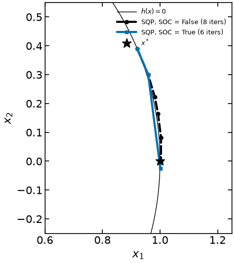

What is not here¶

Trust region SQP (Biegler Section 6.2.3, pp. 148--151; N&W Section 18.5): the composite step / Byrd--Omojokun method, S $\ell_1$ QP, and the filter trust region. Each needs its own step-computation machinery; the lecture develops them, this notebook does not.
Feasibility restoration, which is what would rescue Example 6.3 from $x^0 = [0,0,0,0]^T$ .
Warm starting the QP working set from the previous iteration, which is what makes IQP affordable on real problems.
Reduced-space SQP and sparse linear algebra. Everything above is dense.
General inequalities $g(x) \leq 0$ . They are written as bounds on slacks, which costs no generality (Biegler Section 6.1) but does cost variables.