Your First Optimization Problem - Optimization for Decision Science

Let’s solve your first optimization problem in Pyomo.

Cloud Computing with Google Colab¶

We will include the following code at the top of our notebooks to configure Google Colab.

## Tip: Please put code like this at the top of your notebook.
# We want all of the module/package installations to start up front

import sys

if "google.colab" in sys.modules:
    !wget "https://raw.githubusercontent.com/ndcbe/optimization/main/notebooks/helper.py"
    import helper

    helper.easy_install()
else:
    sys.path.insert(0, "../")
    import helper
helper.set_plotting_style()

What does this code do? If we run it on Google Colab, the code first downloads helper.py. This small utility then helps us install Pyomo and the needed solvers (often via IDAES).

Mathematical Model¶

Let’s start with a purely mathematical example:

\begin{align*} \min_{x} \quad & x_1^2 + 2 x_2^2 - x_3 \\ \mathrm{s.t.} \quad & x_1 + x_2 = 1 \\ & x_1 + 2 x_2 - x_3 = 5 \\ & -10 \leq x_1, x_2, x_3 \leq 10 \end{align*}

(1)

We want to solve the constrained optimization problem numerically.

Define the Model in Pyomo¶

Activity

Fill in the missing constraint.

import pyomo.environ as pyo

# Create instance of concrete Pyomo model.
# concrete means all of the sets and model data are specified at the time of model construction.
# In this class, you'll use a concrete model.
m = pyo.ConcreteModel()

## Declare variables with initial values with bounds
m.x1 = pyo.Var(initialize=1, bounds=(-10, 10))
m.x2 = pyo.Var(initialize=1, bounds=(-10, 10))
m.x3 = pyo.Var(initialize=1, bounds=(-10, 10))

## Declare objective
m.OBJ = pyo.Objective(expr=m.x1**2 + 2 * m.x2**2 - m.x3, sense=pyo.minimize)

## Declare equality constraints
m.h1 = pyo.Constraint(expr=m.x1 + m.x2 == 1)

# Add your solution here

## Display model
m.pprint()

Solve using Ipopt¶

Toward the end of the semester we will learn, in perhaps more detail than you care, what makes Ipopt work under the hood. For now, we’ll use it as a computational tool.

opt1 = pyo.SolverFactory("ipopt")
status1 = opt1.solve(m, tee=True)
assert pyo.check_optimal_termination(status1), (
    f"Solve failed: status={status1.solver.status}, "
    f"termination={status1.solver.termination_condition}"
)

Ipopt 3.14.19: 

******************************************************************************
This program contains Ipopt, a library for large-scale nonlinear optimization.
 Ipopt is released as open source code under the Eclipse Public License (EPL).
         For more information visit https://github.com/coin-or/Ipopt
******************************************************************************

This is Ipopt version 3.14.19, running with linear solver MUMPS 5.8.2.

Number of nonzeros in equality constraint Jacobian...:        5
Number of nonzeros in inequality constraint Jacobian.:        0
Number of nonzeros in Lagrangian Hessian.............:        2

Total number of variables............................:        3
                     variables with only lower bounds:        0
                variables with lower and upper bounds:        3
                     variables with only upper bounds:        0
Total number of equality constraints.................:        2
Total number of inequality constraints...............:        0
        inequality constraints with only lower bounds:        0
   inequality constraints with lower and upper bounds:        0
        inequality constraints with only upper bounds:        0

iter    objective    inf_pr   inf_du lg(mu)  ||d||  lg(rg) alpha_du alpha_pr  ls
   0  2.0000000e+00 3.00e+00 3.33e-01  -1.0 0.00e+00    -  0.00e+00 0.00e+00   0
   1  4.3065612e+00 0.00e+00 2.89e-01  -1.0 4.36e+00    -  6.72e-01 1.00e+00h  1
   2  4.2501103e+00 8.88e-16 1.34e-16  -1.0 1.31e-01    -  1.00e+00 1.00e+00f  1
   3  4.2500000e+00 0.00e+00 4.32e-16  -2.5 6.02e-03    -  1.00e+00 1.00e+00f  1
   4  4.2500000e+00 0.00e+00 1.14e-16  -3.8 4.41e-05    -  1.00e+00 1.00e+00f  1
   5  4.2500000e+00 0.00e+00 1.31e-16  -5.7 1.98e-06    -  1.00e+00 1.00e+00f  1
   6  4.2500000e+00 0.00e+00 3.08e-16  -8.6 2.45e-08    -  1.00e+00 1.00e+00f  1

Number of Iterations....: 6

                                   (scaled)                 (unscaled)
Objective...............:   4.2500000000000000e+00    4.2500000000000000e+00
Dual infeasibility......:   3.0826231515081323e-16    3.0826231515081323e-16
Constraint violation....:   0.0000000000000000e+00    0.0000000000000000e+00
Variable bound violation:   0.0000000000000000e+00    0.0000000000000000e+00
Complementarity.........:   2.5059105039901454e-09    2.5059105039901454e-09
Overall NLP error.......:   2.5059105039901454e-09    2.5059105039901454e-09


Number of objective function evaluations             = 7
Number of objective gradient evaluations             = 7
Number of equality constraint evaluations            = 7
Number of inequality constraint evaluations          = 0
Number of equality constraint Jacobian evaluations   = 7
Number of inequality constraint Jacobian evaluations = 0
Number of Lagrangian Hessian evaluations             = 6
Total seconds in IPOPT                               = 0.092

EXIT: Optimal Solution Found.

Inspect the Solution¶

Now let’s inspect the solution. We’ll use the function value() to extract the numeric value from the Pyomo variable object.

## Return the solution
print("x1 = ", pyo.value(m.x1))
print("x2 = ", pyo.value(m.x2))
print("x3 = ", pyo.value(m.x3))
print("\n")

x1 =  0.49999999996668265
x2 =  0.5000000000333173
x3 =  -3.4999999999666827

Visualize the Solution¶

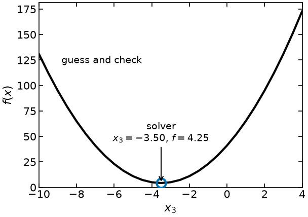
Is our answer correct?

We can solve this optimization problem with guess and check. If we guess $x_3$ , we can then solve the constraints for $x_1$ and $x_2$ :

Constraints:

\begin{align*} & x_1 + x_2 = 1 \\ & x_1 + 2 x_2 - x_3 = 5 \end{align*}

(2)

\begin{bmatrix} 1 & 1 \\ 1 & 2 \end{bmatrix} \begin{bmatrix} x_1 \\ x_2 \end{bmatrix} = \begin{bmatrix} 1 \\ 5 + x_3 \end{bmatrix}

(3)

We can then evaluate the objective. Let’s see the graphical solution to our optimization problem.

Activity

Verify you agree with how to translate the two linear constraints into a linear system of equations.

Objective versus x3 from guess-and-check, with the solver's answer marked

import numpy as np
import matplotlib.pyplot as plt


def constraints(x3):
    """Solve the linear constraints

    Args:
        x3: Value for the decision variable x3

    Returns:
        x1 and x2: Values calculated from the constraints
    """

    # Define the matrices in the above equations
    A = np.array([[1, 1], [1, 2]])
    b = np.array([1, 5 + x3])

    # Solve the linear system of equations
    z = np.linalg.solve(A, b)
    x1 = z[0]
    x2 = z[1]
    return x1, x2


# Define a lambda function to plot the objective
objective = lambda x1, x2, x3: x1**2 + 2 * x2**2 - x3

# Guess many values of x3.
x3_guesses = np.linspace(-10, 4, 21)
obj = []
for x3 in x3_guesses:
    # Solve the constraints to determine x1 and x2
    x1, x2 = constraints(x3)
    # Calculate the store the objective function value
    obj.append(objective(x1, x2, x3))

# Plot the objective function value versus x3
plt.plot(x3_guesses, obj, color="blue", linewidth=2, label="Sensitivity Analysis")
plt.xlabel("$x_3$", fontsize=18)
plt.ylabel("$f(x)$", fontsize=18)

# Plot the solution from Pyomo
x3_sln = pyo.value(m.x3)
obj_sln = pyo.value(m.OBJ)
plt.plot(
    x3_sln,
    obj_sln,
    marker="o",
    color="red",
    markersize=10,
    label="Pyomo Solution",
    linestyle="",
)
plt.legend()
plt.grid(True)
plt.show()