Optimization Modeling with Applications

Taxonomy of Optimization Problems¶

Reference: Chapter 1 in Biegler (2010).

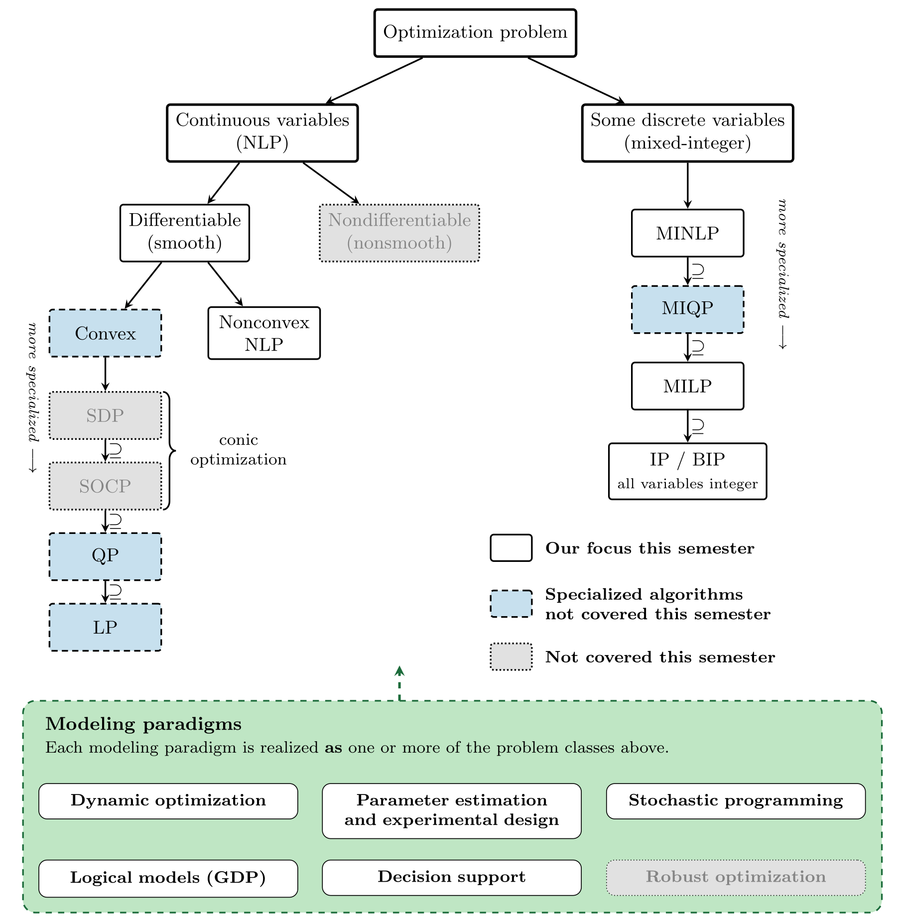
The chart below organizes optimization problems by two questions: are any of the decision variables discrete, and are the objective and constraints differentiable? Those two answers largely determine which algorithms apply, which is why we start here.

Taxonomy of optimization problems. The tree splits on continuous versus discrete variables, then on differentiable versus nondifferentiable. Both branches end in a chain of inclusions read downward from the most general class to the most specific: SDP contains SOCP contains QP contains LP on the convex side, and MINLP contains MIQP contains MILP contains IP on the mixed-integer side. A separate light green band at the bottom lists six modeling paradigms -- dynamic optimization, parameter estimation and experimental design, stochastic programming, logical models, decision support, and robust optimization -- which cut across the tree rather than forming another branch of it; robust optimization carries the same dotted grey not-covered marking the tree uses. A brace labelled conic optimization groups SDP and SOCP. Boxes are shaded and outlined three ways: our focus this semester, specialized algorithms not covered, and not covered.

Three things in this chart are worth pausing on.

Each branch ends in a chain of inclusions, read downward from the most general. On the convex side, every semidefinite program (SDP) contains the second-order cone programs (SOCP) as the case where the matrices are block-diagonal; every SOCP contains the convex quadratic programs (indeed the convex quadratically constrained QPs); and every QP contains the linear programs as the case of a zero Hessian. SOCP and SDP are the conic programs, and this chain is where they fit: they are the natural continuation of LP and QP, not a separate kingdom. We will not cover them, but it is worth knowing the ladder exists — a surprising number of engineering problems (robust design, some control synthesis, relaxations of nonconvex QPs) turn out to be conic once written the right way.

The mixed-integer side nests the same way. MINLP $\supseteq$ MIQP $\supseteq$ MILP $\supseteq$ IP. An MIQP is just an MILP that has been allowed a quadratic objective; it earns a box because it is by far the most common MINLP you will meet in practice (portfolio selection with a cardinality limit, best-subset regression, hybrid MPC with a quadratic cost). We solve MIQPs in this course but do not study algorithms specific to them.

The bottom band is not part of the tree. This is the point students most often miss, and the reason the band is drawn as a different kind of object. Dynamic optimization, parameter estimation and experimental design, stochastic programming, logical models, decision support, and robust optimization are modeling paradigms — ways of writing a problem down. They are orthogonal to the LP/QP/NLP/MINLP axis. Concretely, each one is realized as one of the classes above:

Paradigm	What it becomes once written down
Dynamic optimization (DAEs, collocation)	discretizes into a large NLP — or an MINLP if there are also discrete decisions
Parameter estimation and experimental design	usually an NLP; an MINLP when you are also choosing which experiments to run
Stochastic programming	anything from an LP to an MINLP, only much bigger — one copy of the model per scenario
Logical models (disjunctions, GDP)	reformulates to an MILP or an MINLP
Decision support (multi-objective, bilevel)	wraps any class above in a second layer
Robust optimization (not covered this semester)	depends on the uncertainty set: a box or polyhedral set keeps an LP an LP, while an ellipsoidal set turns it into an SOCP

So a stochastic program may be an LP or an MINLP depending on what is inside it, and a dynamic optimization problem is not a class at all until you discretize it, at which point it becomes a (usually very large) NLP. Robust optimization makes the same point in the other direction: the shape of the uncertainty set, not the application, decides the class — a box or polyhedral set leaves you with an LP, an ellipsoidal one lands you in the SOCPs, which is exactly the conic rung marked not covered above. Each of these paradigms gets its own lecture later in Part I, and in every case the punchline is the same: after the modeling step, you are back in the tree above.

Note

The shading separates two different kinds of “we will not cover this”. Convex, LP, QP, and MIQP are marked specialized algorithms not covered this semester: we formulate and solve these all semester, but the simplex method and specialized convex solvers are not what this course is about — we study algorithms for general nonlinear programs instead. SOCP, SDP, and nondifferentiable optimization are not covered at all, and so is robust optimization in the band below — the band reuses the tree’s own dotted grey marking, so the same legend decodes both. MILP and global optimization, by contrast, are covered.

The brace marks the two conic classes, and it also explains the one thing in the chart that looks like a slip: read down the convex chain and the shading changes twice, at SDP and again at QP. The chain is ordered by mathematical inclusion, the shading by what we cover, and the two orderings simply do not line up.

Adapted from Figure 1.1 of Biegler (2010). The shading, the conic and mixed-integer inclusion chains, and the modeling-paradigm band are additions for this course.

Linear Programs (LP) / Linear Optimization Problems¶

\begin{align*} \min_{x} \quad & f^T x & \text{(linear objective)} \\ \text{s.t.} \quad & A \cdot x = b & \text{(linear constraints)} \\ & x^L \leq x \leq x^U & \text{(bounds)} \end{align*}

(1)

Recall, “s.t.” means “subject to”.

How to enforce $x_1 + x_2 \leq c$ in the above formulation? Convert it to an equality constraint:

x_1 + x_2 = s_1

(2)

where $s_1$ is a slack variable.

Quadratic Program (QP)¶

\begin{align*} \min_{x} \quad & \frac{1}{2} x^T H x + f^T x & \text{(quadratic objective)} \\ \text{s.t.} \quad & A \cdot x = b & \text{(linear constraints)} \\ & x^L \leq x \leq x^U & \text{(bounds)} \end{align*}

(3)

Parameters: $H$ , $f$ , $A$ , $b$ , $x^L$ , $x^U$

There are specialized solvers for LP, QP, and other convex optimization problems. We will not focus on these in this class, but instead consider algorithms for general nonlinear programs.

Nonlinear Program (NLP)¶

\begin{align*} \min_{x} \quad & f(x) & \text{(nonlinear objective)} \\ \text{s.t.} \quad & g(x) = 0 & \text{(equality constraints)} \\ & h(x) \leq 0 & \text{(inequality constraints)} \end{align*}

(4)

where $f(x), g(x), h(x)$ are all nonlinear functions. Bounds can be modeled as inequality constraints.

Mixed Integer Nonlinear Programs (MINLP)¶

The most general form is:

\begin{align*} \min_{x,y} \quad & f(x,y) & \text{(nonlinear objective)} \\ \text{s.t.} \quad & g(x,y) = 0 & \text{(equality constraints)} \\ & h(x,y) \leq 0 & \text{(inequality constraints)} \\ & x \in \mathbb{R}^{n}, ~ y \in \{0,1\}^m \end{align*}

(5)

It is much easier to design algorithms to solve MINLPs with the following structure:

\begin{align*} \min_{x,y} \quad & f(x) + g^T y & \text{(nonlinear objective)} \\ \text{s.t.} \quad & A \cdot x + B \cdot y = c & \text{(linear equality constraints)} \\ & g(x) = 0 & \text{(nonlinear equality constraints)} \\ & h(x) \leq 0 & \text{(nonlinear inequality constraints)} \\ & x \in \mathbb{R}^{n}, ~ y \in \{0,1\}^m \end{align*}

(6)

where x are continuous and y are discrete (binary) variables. Notice y only enters linearly into the objective and equality constraint.

Where These Problem Classes Show Up¶

The table below maps common application areas onto the five problem classes above. Read a row as “problems of this kind are routinely posed as one of these”; most rows have several marks, because the same application admits models at several levels of fidelity, and choosing that level is the modeling decision.

Application	LP	MILP	QP	NLP	MINLP
Model building and data analysis
Parameter estimation / model calibration	✓		✓	✓	✓
Design of experiments		✓		✓	✓
Machine learning: training and inference		✓	✓	✓	✓
Design and synthesis
Heat and mass exchanger networks	✓	✓		✓	✓
Separation sequencing		✓		✓	✓
Reactors and flowsheeting	✓			✓	✓
Facility location and network design	✓	✓			✓
Operations and planning
Production scheduling	✓	✓			✓
Supply chain and logistics	✓	✓			✓
Real-time optimization	✓		✓	✓
Power grid dispatch and unit commitment	✓	✓	✓	✓	✓
Portfolio optimization	✓		✓	✓	✓
Control
Linear model predictive control (MPC)	✓		✓
Nonlinear MPC			✓	✓
Hybrid MPC		✓			✓

A few rows are worth a comment:

Parameter estimation is a QP when the model is linear in the parameters and the objective is least squares; it is an NLP as soon as the model is not; and it is an MINLP when you are also choosing which model to fit. This is the subject of its own lecture.
Machine learning is optimization. Training a support vector machine is a QP; training a neural network is a (very large, nonconvex) NLP; verifying a trained ReLU network, or fitting an optimal decision tree, is an MILP; best-subset regression is a mixed-integer quadratic program.
Power grid dispatch is the one row that touches every column. Economic dispatch with a linear cost curve is an LP and with a quadratic one a QP; unit commitment adds on/off decisions and becomes an MILP; AC optimal power flow is a nonconvex NLP; AC unit commitment is an MINLP. One application, five formulations, chosen by how much physics you keep.
Hybrid MPC is “MPC with discrete actuators” — a valve that is open or shut, a compressor that is on or off — and the discreteness is exactly what pushes it out of QP and into MILP.