This notebook contains material from cbe67701-uncertainty-quantification; content is available on Github.
9.2 Uniform Random Variables: Legendre Polynomials
Created by Kanishka Ghosh (kghosh@nd.edu)
The following text, example, and code have been adapted from:
McClarren, Ryan G (2018). Uncertainty Quantification and Predictive Computational Science: A Foundation for Physical Scientists and Engineers, Chapter 9: Stochastic Collocation and Projection, Springer, https://link.springer.com/chapter/10.1007/978-3-319-99525-0_9
# Download figures (if needed)
import os, requests, urllib

# GitHub pages url
url = "https://ndcbe.github.io/cbe67701-uncertainty-quantification/"

# relative file paths to download
# this is the only line of code you need to change
file_paths = ['figures/Fig-9.4_Table-9.7.png']

# loop over all files to download
for file_path in file_paths:
    print("Checking for",file_path)
    # split each file_path into a folder and filename
    stem, filename = os.path.split(file_path)

    # check if the folder name is not empty
    if stem:
        # check if the folder exists
        if not os.path.exists(stem):
            print("\tCreating folder",stem)
            # if the folder does not exist, create it
            os.mkdir(stem)
    # if the file does not exist, create it by downloading from GitHub pages
    if not os.path.isfile(file_path):
        file_url = urllib.parse.urljoin(url,
                urllib.request.pathname2url(file_path))
        print("\tDownloading",file_url)
        with open(file_path, 'wb') as f:
            f.write(requests.get(file_url).content)
    else:
        print("\tFile found!")
9.2.1 Generalized Polynomial Chaos
Approach to approximate the mapping from input parameter to output random variable using different polynomial expansions when the input parameter is not normally distributed.
Uniform Random Variables: Legendre Polynomials
(adapted from McClarren 2018)
If we consider a random variable $x$ is uniformly distributed in the range $[a,b]$, then $x$ can be written as $x \sim \mathcal{U}[a,b]$ and the PDF of $x$ is given as:
To correspond with the support with the standard definition of Legendre polynomials, the interval $[a,b]$ is mapped to $[-1,1]$ by defining random variable $z$ such that $z \sim \mathcal{U}[-1,1]$. $x$ and $z$ are related as:
Then, the expectation of a uniform random variable $g(x)$ transforms to:
For a function in range $[-1,1]$, the Legendre polynomials form an orthogonal basis and are defined as:
where $n$ is the order of the polynomial.
The expansion of a square-integrable function $g(x)$ on the interval $[a,b]$ in terms of Legrende polynomials is then given as:
where $c_n$ is defined by
\begin{align*} c_n = \frac{2n+1}{2} \int\limits_{-1}^{1}g \left( \frac{b-a}{2}z + \frac{a+b}{2} \right)P_n(z)dz \end{align*}As $P_0(x) = 1$ (from Table 9.6 of text), $c_0$ gives the mean of the expansion $G \sim g(x)$
The variance of the expansion G is equivalent to the sum of the squares of the Legendre polynomial coefficients with $n \geq 1$:
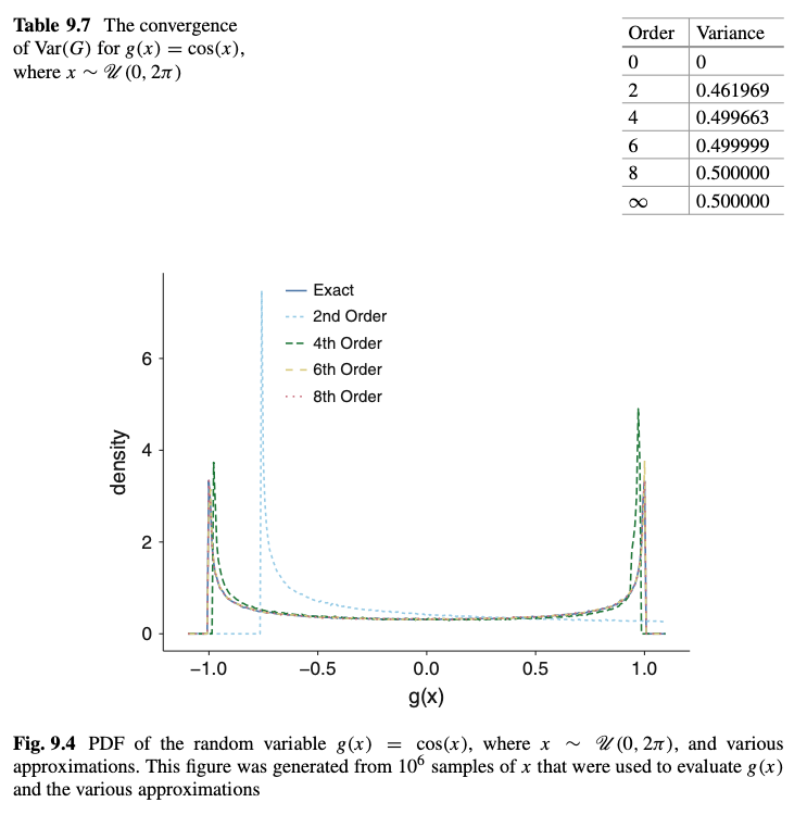
9.2.2 Example: $G \sim g(x) = cos(x)$ and $x \sim \mathcal{U}(0,2\pi)$
The Legendre polynomial coefficients are given as:
The variance of this function is given as:
The $n^{\mathrm{th}}$-order approximations for $G$ using Legendre polynomials can be represented by $G_{approx,n}$ and are calculated as:
and the corresponding variance is given by:
Results from Textbook
Following is a screenshot of the results presented in the text (Pg. 201, Table 9.7 and Fig. 9.4):
Implementation Notes:
- In this implementation,
scipy.specials.eval_legendre()has been used evaluate the $n^{\mathrm{th}}$-order Legendre polynomial https://docs.scipy.org/doc/scipy/reference/generated/scipy.special.eval_legendre.html - To reduce runtime, 1000 samples of $x \sim \mathcal{U}(0,2\pi)$ have been used for the following calculations
9.2.3 Importing libraries
## import all needed Python libraries here
import numpy as np
import pandas as pd
from scipy.stats import uniform
from scipy.special import legendre,eval_legendre
# from scipy.misc import derivative
from scipy import integrate
import matplotlib.pyplot as plt
import seaborn as sns
9.2.4 Functions to calculate exact and $n^{\mathrm{th}}$-order Legendre polynomial approximation of $g(x)$
def g_x_exact(x):
    '''
    Function to create the exact form of the random variable, g(x),
    being approximated
    Argument:
        x: Random variable from uniform distribution U[a,b]
    Return:
        Exact form of the random variable, g(x), being approximated (Here, cos(x))
    '''
    return np.cos(x)

def transform_z_to_x(z,a,b):
    '''
    Helper function to return x in terms of z (Eq. 9.16 of text)
    Arguments:
        z: Random variable from uniform distribution U[-1,1]
        a: Lower limit of uniform random variable x
        b: Upper limit of uniform random variable x
    Returns:
        x: Random variable from uniform distribution U[a,b] in terms of z
    '''
    return ((b-a)/2)*z + (a+b)/2

def transform_x_to_z(x,a,b):
    '''
    Helper function to return z in terms of x (Eq. 9.17 of text)
    Arguments:
        x: Random variable from uniform distribution U[a,b]
        a: Lower limit of uniform random variable x
        b: Upper limit of uniform random variable x
    Returns:
        z: Random variable from uniform distribution U[-1,1] in terms of x
    '''
    return (a+b - 2*x)/(a-b)

def coef_n(a,b,n):
    '''
    Function to generate the Legendre polynomial coefficient of order n
    Argument:
        a: Lower limit of uniform random variable x
        b: Upper limit of uniform random variable x
        n: Order of Legendre polynomial
    Return:
        n-th order Legendre polynomial coefficient (Eq. 9.22 of text)
    '''
    # Create a lambda function to return the integrand in terms of z as shown in
    # Eq. 9.22 of text.
    # Here, scipy.special.eval_legendre() has been used to evaluate the n-th
    # order Legendre polynomial
    # https://docs.scipy.org/doc/scipy/reference/generated/scipy.special.eval_legendre.html
    integrand_func = lambda z: g_x_exact(transform_z_to_x(z,a,b))* \
                               eval_legendre(n,z)
    val,err = integrate.quad(integrand_func,-1,1)
    return ((2*n + 1)/2)* val

def g_x_approximation(x,a,b,n):
    '''
    Function to generate the n-th order Legendre polynomial expansion of the
    random variable g(x), from Eq. 9.21 in text
    Arguments:
        x: Random variable from uniform distribution U[a,b]
        a: Lower limit of uniform random variable x
        b: Upper limit of uniform random variable x
        n: Order of Legendre polynomial
    Return:
        n-th order Legendre polynomial expansion of g(x) (Eq. 9.21 of text)
    '''
    # calculating z in terms of x
    z = transform_x_to_z(x,a,b)
    # n-th order approximation of g(x)
    expansion_sum = 0
    # sum over 0 to n-th order Legendre polynomials following from Eq. 9.21 of text
    for n_ in range(n+1):
        expansion_sum += coef_n(a,b,n_) * eval_legendre(n_,z)
    return expansion_sum
9.2.5 Function to calculate $\mathrm{Var}(g(x))$, $E[G]$, and $\mathrm{Var}(G)$
def var_G_inf(a,b):
    '''
    Function to calculate the infinite-order approximation of variance of g(x)
    following Eq. 9.27 of text
    Arguments:
        a: Lower limit of uniform random variable x
        b: Upper limit of uniform random variable x
    Return:
        Variance of g(x)
    '''
    # Var(g(x))
    # lambda function to define integrand g(x)^2
    integrand_func = lambda x: g_x_exact(x)**2
    val, err = integrate.quad(integrand_func,a,b)
    return (1/(b-a)) * val

def mean_G(a,b):
    '''
    Function to calculate the mean of the Legendre polynomial expansion G of g(x)
    following Eq. 9.23 of text
    Arguments:
        a: Lower limit of uniform random variable x
        b: Upper limit of uniform random variable x
    Return:
        Variance of G
    '''
    # lambda function to define integrand g(x)
    integrand_func = lambda x: g_x_exact(x)
    val, err = integrate.quad(integrand_func,a,b)
    return (1/(b-a)) * val

# function to calculate variance of G ~ g(x)
def var_G_approximation(a,b,n):
    '''
    Function to calculate the variance of the n-th order Legendre polynomial
    expansion of g(x) following Eq. 9.24 of text
    Arguments:
        a: Lower limit of uniform random variable x
        b: Upper limit of uniform random variable x
        n: Highest order of Legendre polynomial used for the
    Return:
        Variance of n-th order Legendre polynomial expansion G of g(x)
    '''
    # Var(G(approx,n))
    sum_sq_coef = 0
    # sum of the squares coefficients with n  >= 1
    for n_ in range(n+1):
        if n_ == 0:
            pass
        else:
            sum_sq_coef += (1/(2*n_ + 1))*coef_n(a,b,n_)**2
    return sum_sq_coef
9.2.6 Generating samples from $\mathcal{U}[0,2\pi]$
# Number of samples to dram from uniform distribution (1000 samples to reduce computation time)
n_samples = 1000
# Lower bound of interval for x~ U[0,2pi]
a = 0
# Upper bound of interval for x~ U[0,2pi]
b = 2*np.pi
# Orders of Legendre polynomials used for the approximation
n_vals = [0,2,4,6,8]
# n_samples number of samples drawn from U[0,1)
uniform_samples = np.random.random_sample(n_samples)
# Samples of x drawn from uniform distribution U[0,2pi)
x_vals = [(b - a) * u_samp + a for u_samp in uniform_samples]
9.2.7 Convergence of variance for $g(x) = cos(x)$, where $ x \sim \mathcal{U} (0, 2\pi )$
# List to store variance of Legendre polynomial approximations of g(x)
var_G_list = []
# List to store order of approximations of g(x) as strings
n_val_list = []

# Loop through the different order-cases which are used to approximate g(x)
for n in n_vals:
    # Calculate variance for n-order approximation of g(x)
    var_G_approx_n = var_G_approximation(a,b,n)
    # Store n-order approximation in variance list
    var_G_list.append(var_G_approx_n)
    # Store string format of order of approximation in order list
    n_val_list.append(str(n))

# Calculate infinite-order variance of g(x)
var_G = var_G_inf(a,b)
# Add infinite-order variance to variance list
var_G_list.append(var_G)
# Add order infinity to order list
n_val_list.append('Infinity')

# Create a pandas dataframe to display the converge of Var(G)
variance_data = {'Order':n_val_list,'Variance':var_G_list}
df_to_print = pd.DataFrame(variance_data,columns=['Order','Variance'])
df_to_print
9.2.8 Approximate $g(x)$ using different orders of Legendre polynomials
# Evaluate exact values (order = infinity) of g(x) for samples of x generated
g_x_exact_vals = [g_x_exact(x) for x in x_vals]

# Evaluate 2nd-order approximation of g(x) for samples of x generated
g_x_approx_n_2 = [g_x_approximation(x,a,b,2) for x in x_vals]

# Evaluate 4th-order approximation of g(x) for samples of x generated
g_x_approx_n_4 = [g_x_approximation(x,a,b,4) for x in x_vals]

# Evaluate 6th-order approximation of g(x) for samples of x generated
g_x_approx_n_6 = [g_x_approximation(x,a,b,6) for x in x_vals]

# Evaluate 8th-order approximation of g(x) for samples of x generated
g_x_approx_n_8 = [g_x_approximation(x,a,b,8) for x in x_vals]
9.2.9 Plot PDF of the random variable $g(x) = \cos(x)$, where $x \sim \mathcal{U}(0, 2\pi)$, and various approximations
# Plot the distributions
plt.figure(figsize=(8,6))
# Exact values
sns.distplot(g_x_exact(x_vals),
             kde_kws = {'linewidth': 2,'label' : 'Exact'},
             hist_kws = {'alpha':0.25,'linewidth':2})
# Order 2 approximation
sns.distplot(g_x_approx_n_2,
             kde_kws = {'linewidth': 2,'linestyle':'dashed','label' : '2nd order'},
             hist_kws = {'alpha':0.25,'linewidth':1})
# Order 4 approximation
sns.distplot(g_x_approx_n_4,
             kde_kws = {'linewidth': 2,'linestyle':'dashdot','label' : '4th order'},
             hist_kws = {'alpha':0.25,'linewidth':1})
# Order 6 approximation
sns.distplot(g_x_approx_n_6,
             kde_kws = {'linewidth': 2,'linestyle':'dashed','label' : '6th order'},
             hist_kws = {'alpha':0.25,'linewidth':1})
# Order 8 approximation
sns.distplot(g_x_approx_n_8,
             kde_kws = {'linewidth': 2,'linestyle':'dashdot','label' : '8th order'},
             hist_kws = {'alpha':0.25,'linewidth':1})

plt.xlim(-1.75,1.75)
plt.xlabel('$g(x)$', fontsize = 17)
plt.ylabel('density', fontsize = 17)
plt.xticks([-1,-0.5,0,0.5,1], fontsize = 17)
plt.title('PDF of various approximations of random variable $g(x) = \cos(x)$ \n $x \sim \mathcal{U}(0,2\pi)$',fontsize = 17)
plt.grid()
plt.legend(loc='upper center',bbox_to_anchor=(0.5, -0.2),ncol=3,fontsize = 17)
plt.show()

Note: The second order approximation returns $\cos(x)$ values in excess of 1. I am not sure why this is happening (similar behavior can be seen in Fig. 9.4 in the text)