# Load required Python libraries.
import matplotlib.pyplot as plt
import numpy as np
from scipy import linalg
from matplotlib import cm
Eigenvalues and Quadratic Programs
Main Idea: By looking at an unconstrained quadratic optimization problem, we will see how the eigenvalues tell us about the curvature (second derivatives) and help us classify the stationary points.
Reference: Section 2.2.2 Quadratic Forms in Biegler (2010)
For the symmetric quadratic , rotate into the eigenvector coordinates of . The eigenvalue signs then classify the geometry:
| Curvature of | Stationary point | Global behavior |
|---|---|---|
| positive definite | unique minimum | bounded below |
| negative definite | unique maximum | bounded above |
| positive/negative semidefinite | continuum of optima, if a stationary point exists | flat directions |
| indefinite | saddle point, if nonsingular | unbounded above and below |
| indefinite and singular | continuum of saddle points, if a stationary point exists | unbounded above and below |
| singular with a linear term in a null-space direction | no stationary point | unbounded in that direction |
See Biegler (2010), Section 2.2.2, pp. 22--25.
Analysis Algorithm
We will start by defining a function for our classification procedure.
# The main event
def quad_analyze(c, a, B):
    """
    Analyze the stationary points of a quadratic objective.

    Inputs:
        c - offset (scalar)
        a - linear coefficients (vector)
        B - quadratic coefficients (matrix)

    Outputs:
        None

    Displayed:
        1. Inputs
        2. Eigenvalues and eigenvectors
        3. Stationary point (transformed coordinates)
        4. Stationary point (original coordinates)
        5. Function value and gradient at stationary point
        6. 3D plot
    """

    ### Display inputs
    print("***Inputs***")
    print("c = ", c, "\n")
    print("a = ", a, "\n")
    print("B = \n", B, "\n")

    ### Eigendecomposition
    print("***Eigendecomposition***")
    l, V = linalg.eig(B)
    print("Lambda = \n", np.diag(l), "\n")
    print("V = \n", V, "\n")

    ### Calculate stationary point
    n = len(a)
    zstar = np.zeros(n)

    abar = (V.transpose()).dot(a)
    print("abar = \n", abar, "\n")

    # Loop over dimensions
    for j in range(0, n):
        # If eigenvalue is NOT zero
        ##
        # Previous code
        # if(l[j] != 0):
        ##
        # More stable version
        if abs(l[j]) > 1e-8:
            zstar[j] = -abar[j] / np.real(l[j])

        # Otherwise check if abar is nonzero
        elif abar[j] != 0:
            print("WARNING: No stationary point exists.")

    xstar = V.dot(zstar)

    print("***(Possible) Stationary Point in Transformed Coordinates:")
    print("z* = ", zstar, "\n")

    print("***(Possible) Stationary Point in Original Coordinates:")
    print("x* = ", xstar, "\n")

    ### Check function value and gradient
    fval = c + a.dot(xstar) + 0.5 * xstar.dot(B.dot(xstar))
    grad = a + xstar.dot(B)

    print("***Checking function and gradient***")
    print("f(x*) = ", fval)
    print("f'(x*) = \n", grad, "\n")

    ### Make 3D plot
    # Tutorial: https://matplotlib.org/mpl_toolkits/mplot3d/tutorial.html
    if n == 2:
        # Create vectors in both dimensions
        dx = 5
        x1 = np.arange(xstar[0] - dx, xstar[0] + dx, 0.25)
        x2 = np.arange(xstar[1] - dx, xstar[1] + dx, 0.25)

        # Create a matrix of all points to sample
        X1, X2 = np.meshgrid(x1, x2)
        n1 = len(x1)
        n2 = len(x2)
        F = np.zeros([n2, n1])
        xtemp = np.zeros(2)
        for i in range(0, n1):
            xtemp[0] = x1[i]
            for j in range(0, n2):
                xtemp[1] = x2[j]
                F[j, i] = c + a.dot(xtemp) + 0.5 * xtemp.dot(B.dot(xtemp))

        # Create 3D figure
        fig = plt.figure()
        ax = fig.add_subplot(projection="3d")

        # Plot f(x). viridis is monotone in luminance, so the surface still
        # reads when the handout is printed in black and white. See
        # figures/README.md: coolwarm is not allowed for this reason.
        ax.plot_surface(X1, X2, F, linewidth=0, cmap=cm.viridis, antialiased=True)

        # Add (possible) stationary point
        ax.scatter(
            xstar[0],
            xstar[1],
            fval,
            s=50,
            color="#D55E00",
            marker="o",
            edgecolors="black",
            linewidths=0.8,
            depthshade=True,
        )

        # Draw vertical line through stationary point to help visualization
        # Maximum value in array
        fmax = np.amax(F)
        fmin = np.amin(F)
        ax.plot(
            [xstar[0], xstar[0]],
            [xstar[1], xstar[1]],
            [fmin, fmax],
            color="#D55E00",
            linestyle="--",  # Dashed: a guide line, not part of the surface
        )

        ax.set_xlabel("$x_1$")
        ax.set_ylabel("$x_2$")
        ax.set_zlabel("$f(x)$")

        plt.show()
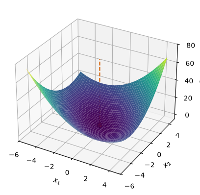
Example 2.8 in Biegler (2010)
c = 0
a = np.array([1, 1])
B = np.array([[2, 1], [1, 2]])

quad_analyze(c, a, B)
***Inputs***
c = 0
a = [1 1]
B =
[[2 1]
[1 2]]
***Eigendecomposition***
Lambda =
[[3.+0.j 0.+0.j]
[0.+0.j 1.+0.j]]
V =
[[ 0.70710678 -0.70710678]
[ 0.70710678 0.70710678]]
abar =
[1.41421356 0. ]
***(Possible) Stationary Point in Transformed Coordinates:
z* = [-0.47140452 -0. ]
***(Possible) Stationary Point in Original Coordinates:
x* = [-0.33333333 -0.33333333]
***Checking function and gradient***
f(x*) = -0.3333333333333333
f'(x*) =
[2.22044605e-16 2.22044605e-16]
Activity 1
Classify the stationary point for .
# Add your solution hereActivity 2
Classify the stationary point for .
Hint: needs to be symmetric.
# Add your solution hereClassifying Functions (Key Concepts from Real Analysis)
Taylor Series Approximation
Finite Difference Approximation
Main Idea: This example complements the in-class example where we use Taylor series expansions to estimate truncation error for forward, backward, and central finite difference formulas. We will revisit finite difference formulas again in a few lectures.
# Define the test function
def my_f(x):
    return np.exp(x)


# Specify point to examine
a = 1.0

# Calculate function value at x = a
fa = my_f(a)

# Calculate exact first derivative at x=1
df1 = my_f(a)  # Need to replace if you consider a different test function!

# Generate values for epsilon
eps = np.power(10, np.arange(-16, 1, 0.25))
n = len(eps)# Preallocate error array
error_forward = np.zeros(n)
# Calculate finite difference approximation and error
for i in range(0, n):
df1_forward = (my_f(a + eps[i]) - fa) / eps[i]
error_forward[i] = abs(df1_forward - df1)
# Plot
plt.figure()
plt.loglog(eps, error_forward, label="Forward", color="black", linestyle="-")
plt.xlabel(r"$\epsilon$")
plt.ylabel("Absolute Error")
plt.legend()
plt.grid()
plt.show()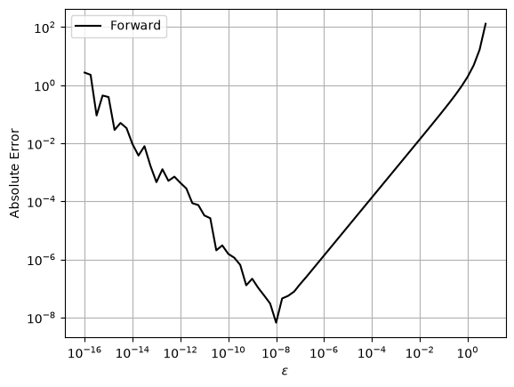
# Preallocate error array
error_backward = np.zeros(n)

# Calculate finite difference approximation and error
for i in range(0, n):
    df1_backward = (fa - my_f(a - eps[i])) / eps[i]
    error_backward[i] = abs(df1_backward - df1)

# Plot
plt.figure()
plt.loglog(eps, error_forward, label="Forward", color="black", linestyle="-")
plt.loglog(eps, error_backward, label="Backward", color="#0072B2", linestyle="--")
plt.xlabel(r"$\epsilon$")
plt.ylabel("Absolute Error")
plt.grid()
plt.legend()
plt.show()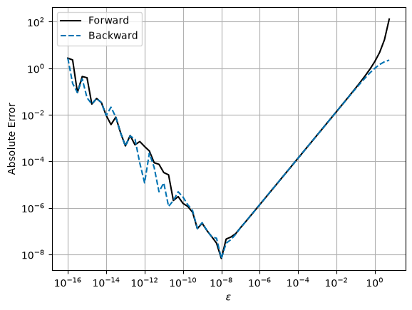
# Preallocate error array
error_central = np.zeros(n)

# Calculate finite difference approximation and error
for i in range(0, n):
    df1_central = (my_f(a + eps[i]) - my_f(a - eps[i])) / (2 * eps[i])
    error_central[i] = abs(df1_central - df1)

# Plot
plt.figure()
plt.loglog(eps, error_forward, label="Forward", color="black", linestyle="-")
plt.loglog(eps, error_backward, label="Backward", color="#0072B2", linestyle="--")
plt.loglog(eps, error_central, label="Central", color="#E69F00", linestyle="-.")
plt.xlabel(r"$\epsilon$")
plt.ylabel("Absolute Error")
plt.grid()
plt.legend()
plt.show()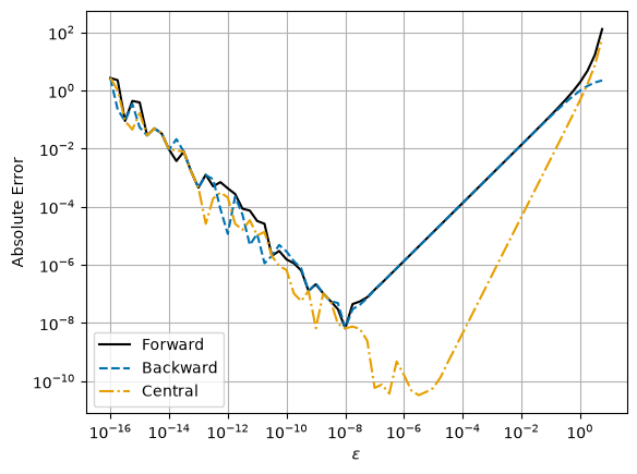
Activity
Record the results for the test function at .
Try the point and record the results.
Try a different test function.
Original: at 
Forward: Lowest absolute error of 10-8 at = 10-8
Backward: Lowest absolute error of 10-8 at = 10-8
Central: Lowest absolute error of 10-10 at = 10-6
Variant: at 
Forward: Lowest absolute error of 10-4 at = 10-8
Backward: Lowest absolute error of 10-4 at = 10-8
Central: Lowest absolute error of 10-6 at = 10-5
Discussion
Are there any general trends from these (limited) computational experiments?
What is the best for an arbitrary function?