Optimizing Experiments with Pyomo.DoE - Optimization for Decision Science

Prepared by: Jialu Wang, Prof. Alex Dowling, Hailey Lynch, and Andrew Marquardt (amarquar@nd.edu, 2024) at the University of Notre Dame.

Introduction and Learning Objectives¶

This notebook uses design of experiments for a reactor kinetics experiment with Pyomo.DoE. The user will be able to learn concepts involved in Model-Based Design of Experiments (MBDoE) and practice using Pyomo.DoE from methodology in the notebook. Results will be interpreted throughout the notebook to connect the material with the Pyomo implementation.

The general process we will follow throughout this notebook:

Import Modules
- Step 0: Import Pyomo and Pyomo.DoE Module
Problem Statement
- Step 1: Mathematical Model for the Reaction Kinetics Example
Implementation in Pyomo
- Step 2: Implement Mathematical Model
- Step 3: Generate an Experiment
- Step 4: Run the DOE Module to get Optimal Design Parameters
Methodology
- Step 5: Method for Computing FIM
- Step 6: Running a Full Factorial Design Experiment
Visualizing Results
- Step 7: Evaluating the Full Factorial Heat Maps
Key Takeaways

Step 0: Import Pyomo and Pyomo.DoE Module¶

# IPOPT installer
import sys

if "google.colab" in sys.modules:
    !wget "https://raw.githubusercontent.com/ndcbe/optimization/main/notebooks/helper.py"
    import helper

    helper.install_idaes()
    helper.install_ipopt()
else:
    sys.path.insert(0, "../")
    import helper

    # Import solver
    import idaes
helper.set_plotting_style()

# Imports
import matplotlib.pyplot as plt
import numpy as np
import pyomo.environ as pyo
from pyomo.contrib.doe import DesignOfExperiments, ObjectiveLib
from pyomo.contrib.parmest.experiment import Experiment
from pyomo.dae import ContinuousSet, DerivativeVar

Step 1: Mathematical Model for the Reaction Kinetics Example¶

Reaction Kinetics¶

Consider two chemical reactions that convert molecule $A$ to desired product $B$ and a less valuable side-product $C$ :

A \overset{k_1}{\rightarrow} B \overset{k_2}{\rightarrow} C

(1)

Goal:

Design a large-scale continuous reactor that maximizes the production of $B$ .

The rate laws for these two chemical reactions are:

r_A = -k_1 C_A

(2)

r_B = k_1 C_A - k_2 C_B

(3)

r_C = k_2 C_B

(4)

Here, $C_A$ , $C_B$ , and $C_C$ are the concentrations of each species.

The rate constants $k_1$ and $k_2$ depend on temperature as follows:

k_1 = A_1 \exp \left({\frac{-1000 E_1}{R T}} \right)

(5)

k_2 = A_2 \exp \left({\frac{-1000 E_2}{R T}}\right)

(6)

where:

$A_1$ [ $\mathrm{hr}^{-1}$ ], $A_2$ [ $\mathrm{hr}^{-1}$ ], $E_1$ [ $kJ/mol$ ], and $E_2$ [ $kJ/mol$ ] are fitted model parameters.
$R$ [ $J/mol K$ ] is the ideal-gas constant.
$T$ [ $K$ ] is absolute temperature.

Objective:

Using the Pyomo ecosystem, we would like to perform uncertainty quantification and design of experiments on a small-scale batch reactor to infer parameters $A_1$ , $A_2$ , $E_1$ , and $E_2$ .

Batch Reactor¶

The concentrations in a batch reactor evolve with time and are modeled by the following differential equations:

\frac{d C_A}{dt} = r_A = -k_1 C_A(t)

(7)

\frac{d C_B}{dt} = r_B = k_1 C_A(t) - k_2 C_B(t)

(8)

\frac{d C_C}{dt} = r_C = k_2 C_B(t)

(9)

We have now established a linear system of differential equations. Next we can write our initial conditions where we assume the feed is only species $A$ such that:

C_A(t=0) = C_{A0}, \quad C_B(t=0) = 0, \quad C_C(t=0) = 0

(10)

When $k_1$ and $k_2$ are at constant temperature, we have the following analytic solution:

C_A(t) = C_{A0} \exp(-k_1 t)

(11)

C_B(t) = \frac{k_1}{k_2 - k_1} C_{A0} \left[\exp(-k_1 t) - \exp(-k_2 t) \right]

(12)

C_C(t) = C_{A0} - \frac{k_2}{k_2 - k_1} C_{A0} \exp(-k_1 t) + \frac{k_1}{k_2 - k_1} \exp(-k_2 t) C_{A0} = C_{A0} - C_{A}(t) - C_{B}(t)

(13)

See the following for more information on batch reactors:

Batch Reactor: AIChE / Wikipedia

Step 2: Implement Mathematical Model¶

This mathematical model is comprised of a system of differential algebraic equations (DAEs). This system will be solved using Pyomo.DAE.

See the following notebooks from CBE 60499 regarding Pyomo.DAE:

The experiment class follows Pyomo’s Experiment interface:

create_model() builds the equations and variables.
finalize_model() fixes nominal parameters, applies collocation, and completes the square simulation model.
label_model() attaches the four required suffixes: experiment inputs, experiment outputs, unknown parameters, and measurement errors.
get_labeled_model() returns the finished model to Pyomo.DoE.

The suffix values have specific meanings. Unknown-parameter values are nominal values, and measurement_error stores the measurement standard deviation, not its variance or a least-squares weight. Here each concentration measurement has standard deviation 0.01 mol/L.

class ReactorExperiment(Experiment):
    def __init__(
        self,
        t_control=None,
        control_val=None,
        t_range=None,
        CA_init=5,
        C_init=None,
        theta_pe=None,
        NFE=32,
        ncp=3,
    ):
        """
        Arguments:
        ---------
        t_control: time-dependent design (control) variables, a list of control timepoints
        control_val: control design variable values T at corresponding timepoints
        t_range: time range, h
        CA_init: time-independent design (control) variable, an initial value for CA
        C_init: An initial value for C
        theta_pe: optimized parmest parameters for the arrhenius kinetic equations
        NFE: number of finite elements in the discretizer
        ncp: number of collocation points per finite element in the discretizer
        """
        if t_control is None:
            t_control = [0, 0.125, 0.25, 0.375, 0.5, 0.625, 0.75, 0.875, 1]
        if control_val is None:
            control_val = [500, 300, 300, 300, 300, 300, 300, 300, 300]
        if t_range is None:
            t_range = [0, 1]
        if C_init is None:
            C_init = [5, 0, 0]
        if theta_pe is None:
            theta_pe = {"A1": 85, "A2": 370, "E1": 8, "E2": 15}

        self.t_range = t_range
        self.CA_init = CA_init
        self.C_init = C_init
        self.NFE = NFE
        self.ncp = ncp
        self.t_control = t_control
        self.control_val = control_val
        self.theta_pe = theta_pe
        self.model = None

    def create_model(self):
        # model build
        m = self.model = pyo.ConcreteModel()

        # concentration intialization
        m.CA_init = self.CA_init

        # Time-independent design variable
        m.t0 = pyo.Set(initialize=[0])
        m.CA0 = pyo.Var(
            m.t0, initialize=self.CA_init, bounds=(0, 5.0), domain=pyo.NonNegativeReals
        )  # mol/L

        # parameters
        m.R = pyo.Param(mutable=False, initialize=8.314)

        # variables
        m.t = ContinuousSet(bounds=(self.t_range[0], self.t_range[1]))

        # Parameter list
        para_list = ["A1", "A2", "E1", "E2"]
        m.para_list = para_list
        # Define parameters as Param
        m.A1 = pyo.Var(domain=pyo.NonNegativeReals)
        m.A2 = pyo.Var(domain=pyo.NonNegativeReals)
        m.E1 = pyo.Var(domain=pyo.NonNegativeReals)
        m.E2 = pyo.Var(domain=pyo.NonNegativeReals)

        # Concentration variables under perturbation
        m.C_set = pyo.Set(initialize=["CA", "CB", "CC"])
        m.CA = pyo.Var(m.t, initialize=self.C_init[0], domain=pyo.NonNegativeReals)
        m.CB = pyo.Var(m.t, initialize=self.C_init[1], domain=pyo.NonNegativeReals)
        m.CC = pyo.Var(m.t, initialize=self.C_init[2], domain=pyo.NonNegativeReals)

        # Time derivatives
        m.dCAdt = DerivativeVar(m.CA, wrt=m.t)
        m.dCBdt = DerivativeVar(m.CB, wrt=m.t)
        m.dCCdt = DerivativeVar(m.CC, wrt=m.t)

        # Time-dependent design variable, initialized with the first control value
        m.t_control = self.t_control
        # Control time points
        m.t_con = pyo.Set(initialize=m.t_control)
        # Controls
        controls = {}
        for i, t in enumerate(self.t_control):
            controls[t] = self.control_val[i]

        def T_initial(m, t):
            if t in m.t_con:
                return controls[t]
            else:
                # count how many control points are before the current t;
                # locate the nearest neighbouring control point before this t
                j = -1
                for t_con in m.t_con:
                    if t > t_con:
                        j += 1
                neighbour_t = m.t_control[j]
                return controls[neighbour_t]

        m.T = pyo.Var(
            m.t, initialize=T_initial, bounds=(300, 700), domain=pyo.NonNegativeReals
        )

        m.kp1 = pyo.Var(m.t, domain=pyo.NonNegativeReals)
        m.kp2 = pyo.Var(m.t, domain=pyo.NonNegativeReals)

        @m.Constraint(m.t)
        def kp1_cons(m, t):
            return m.kp1[t] == m.A1 * pyo.exp(-m.E1 * 1000 / (m.R * m.T[t]))

        @m.Constraint(m.t)
        def kp2_cons(m, t):
            return m.kp2[t] == m.A2 * pyo.exp(-m.E2 * 1000 / (m.R * m.T[t]))

        @m.Constraint(m.C_set, m.t)
        def dCdt_rule(m, y, t):
            """
            Calculate CA in Jacobian matrix analytically

            Arguments:
            y: CA, CB, CC
            t: timepoints

            Return:
            m: Pyomo model
            """
            if y == "CA":
                return m.dCAdt[t] == -m.kp1[t] * m.CA[t]
            elif y == "CB":
                return m.dCBdt[t] == m.kp1[t] * m.CA[t] - m.kp2[t] * m.CB[t]
            elif y == "CC":
                return m.dCCdt[t] == m.kp2[t] * m.CB[t]

        @m.Constraint(m.t)
        def alge(m, t):
            """
            The algebraic equation for mole balance

            Arguments:
            t: time

            Return:
            m: Pyomo model
            """
            return m.CA[t] + m.CB[t] + m.CC[t] == m.CA0[0]

    def finalize_model(self):
        m = self.model

        # fix Arrhenius parameters (any changes necessary will be done automatically by pyomo- this is necessary to ensure that the model DoF is 0)
        m.A1.fix(self.theta_pe["A1"])
        m.A2.fix(self.theta_pe["A2"])
        m.E1.fix(self.theta_pe["E1"])
        m.E2.fix(self.theta_pe["E2"])

        # fix the starting concentration value (similar to Arrhenius parameters, though not strictly necessary in the same way)
        m.CA0.fix(self.CA_init)

        # Boundary Conditions
        m.CB[0.0].fix(0.0)
        m.CC[0.0].fix(0.0)

        @m.Constraint(m.t)
        def T_control(m, t):
            """
            T at interval timepoint equal to the T of the control time point at the beginning of this interval
            Count how many control points are before the current t;
            locate the nearest neighbouring control point before this t

            Arguments:
            m: model
            t: time

            Return:
            m: Pyomo model
            """
            if t in m.t_con:
                return pyo.Constraint.Skip
            else:
                j = -1
                for t_con in m.t_con:
                    if t > t_con:
                        j += 1
                neighbour_t = m.t_control[j]
                return m.T[t] == m.T[neighbour_t]

        # Discretization
        discretizer = pyo.TransformationFactory("dae.collocation")
        discretizer.apply_to(m, nfe=self.NFE, ncp=self.ncp, wrt=m.t)
        for t in m.t:
            m.dCdt_rule["CC", t].deactivate()

    def label_model(self):
        m = self.model

        # Concentration measurement labels
        m.experiment_outputs = pyo.Suffix(direction=pyo.Suffix.LOCAL)
        m.experiment_outputs.update((m.CA[t], None) for t in m.t_control)
        m.experiment_outputs.update((m.CB[t], None) for t in m.t_control)
        m.experiment_outputs.update((m.CC[t], None) for t in m.t_control)

        # measurement values
        m.measurement_error = pyo.Suffix(direction=pyo.Suffix.LOCAL)
        m.measurement_error.update((m.CA[t], 0.01) for t in m.t_control)
        m.measurement_error.update((m.CB[t], 0.01) for t in m.t_control)
        m.measurement_error.update((m.CC[t], 0.01) for t in m.t_control)

        # Design variables
        m.experiment_inputs = pyo.Suffix(direction=pyo.Suffix.LOCAL)
        m.experiment_inputs.update((m.CA0[t], None) for t in m.t0)
        m.experiment_inputs.update((m.T[t], None) for t in m.t_control)

        # unkown parameter labels
        m.unknown_parameters = pyo.Suffix(direction=pyo.Suffix.LOCAL)
        m.unknown_parameters.update((k, pyo.value(k)) for k in [m.A1, m.A2, m.E1, m.E2])

    def get_labeled_model(self):
        if self.model is None:
            self.create_model()
            self.finalize_model()
            self.label_model()
        return self.model

Step 3: Generate an Experiment¶

Recall the unknown model parameters, $\theta = (A_1, A_2, E_1, E_2)$ .

Our goal is to maximize the precision of $\theta$ by measuring the model outputs called $y$ for the initial conditions at each time point such that $y(t)=(C_A(t), C_B(t), C_C(t))$ .

The code block below generates an experiment and then runs the DOE module on the generated experiment class. It uses a relative perturbation of 0.001 and central differences. Central differences are second-order accurate for a smooth response, but 0.001 is a starting value rather than a universal choice: a sensitivity check should confirm that truncation and roundoff errors are acceptably balanced for this model.

experiment = ReactorExperiment()
doe_obj = DesignOfExperiments(
    experiment=experiment,
    fd_formula="central",
    step=1e-3,
    objective_option=ObjectiveLib.determinant,
    scale_constant_value=1.0,
    scale_nominal_param_value=True,
    improve_cholesky_roundoff_error=True,
    tee=False,
)

Step 4: Configure Pyomo.DoE¶

The DesignOfExperiments object now holds the labeled experiment, finite-difference settings, scaling convention, objective, and solver options. We will first inspect the FIM at the nominal design, then explore the design space, and optimize only once at the end.

The design variables are the initial concentration and the piecewise-constant temperature profile. Pyomo.DoE will maximize the selected FIM criterion subject to the dynamic model and design bounds.

This is a local design: the sensitivities and FIM are evaluated near the nominal Arrhenius parameters supplied to the experiment.

Understanding the Output for Running an Experiment¶

The next section connects the software output to determinants, eigenvalues, and the FIM. Useful refreshers are:

Fisher Information Matrix (FIM):¶

Objective:

The FIM measures the information content for the unknown parameters $\theta$ from the model output $y_i$ such that:

y_i=f(\psi_i, \theta)

(14)

In order to quantify the uncertainty of the estimated parameters for parameter estimation, consider the covariance matrix for the parameters:

V(\hat{\theta},\psi) = \left[\sum_{r}^{N_{r}}\sum_{r'}^{N_{r}} \tilde{\sigma}_{(r,r')}Q_{r}^{T}Q_{r'}+V_{\theta}(\hat{\theta})^{-1}\right]^{-1}

(15)

where:

$\hat{\theta}$ : estimated parameters.
$\tilde{\sigma}$ : element in the inverse of the observational covariance matrix.
$r,$ $r'$ : measurements.
$Q$ : dynamic sensitivity.
$V_{\theta}$ : prior information.

The inverse of $V$ estimates the FIM such that:

V(\hat{\theta},\psi) = [M(\hat{\theta},\psi)]^{-1}

(16)

where:

$\psi$ : design vector from a DAE system

For sequential design of experiments, consider prior information such that after $N_e$ experiments, the FIM is calculated by:

M= \sum_{k=1}^{N_e-1}M_k+M_{N_e}(\hat{\theta},\psi_{N_e}) = K+M_{N_e}(\hat{\theta},\psi_{N_e})

(17)

where:

$N_e - 1$ : previous experiments
$K$ : constant matrix encoding information from all $N_e - 1$

Key Takeaways: In regards to parameter estimation,

A large FIM value denotes more information about $\theta$ is gained from the model.

See the following notebook from CBE 60258 for more information on FIM:

Computing FIM

Step 5: Method for Computing FIM¶

This method computes a FIM-based MBDoE optimization problem with no degrees of freedom.

Optimality Conditions¶

In our results, we will use the five optimality conditions below:

Optimality Condition	Definition	Computation	Geometry
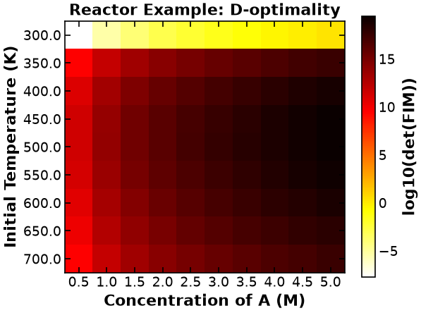
D-Optimality	Maximizes the determinant of $M$ or minimizes the determinant of $V$	Determinant	Minimizes the volume of the confidence ellipsoid
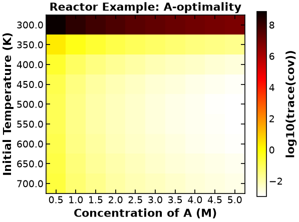
A-Optimality	Minimizes the trace of $V$ , equivalently $\mathrm{trace}(M^{-1}) = \sum_i 1/\lambda_i$	Trace of the inverse	Reduces average marginal variance and emphasizes poorly informed directions
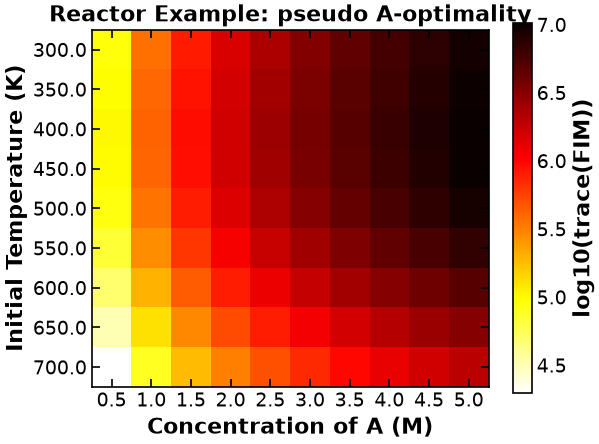
Pseudo-A-Optimality	Maximizes the trace of $M$ , i.e. $\sum_i \lambda_i$ . Not equivalent to A-optimality	Trace	Dominated by the largest eigenvalue; a numerically cheap surrogate
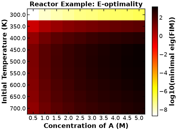
E-Optimality	Maximizes $\lambda_{\min}(M)$ , equivalently minimizing the largest covariance eigenvalue	Minimum eigenvalue	Reduces uncertainty in the least-informed parameter combination and the confidence ellipsoid’s major axis
Modified E-Optimality	Minimizes $\lambda_{\max}(M)/\lambda_{\min}(M)$	Condition number	Reduces directional imbalance (ellipsoid eccentricity) without necessarily increasing total information

Note on A-optimality. Maximizing $\mathrm{trace}(M)$ is not the same as A-optimality, although it is often identified as such. A-optimality minimizes $\mathrm{trace}(M^{-1}) = \sum_i 1/\lambda_i$ , which is dominated by the smallest eigenvalue, so it prioritizes poorly-informed directions. Maximizing $\mathrm{trace}(M) = \sum_i \lambda_i$ is dominated by the largest eigenvalue and is called pseudo-A-optimality; it is cheap because it needs no inversion or eigenvalues. See Laky, Lilonfe, Martin, Klise, Nicholson, Siirola & Dowling, Optimal experimental design using eigenvalue-based criteria with Pyomo.DoE, Digital Discovery (2026), DOI 10.1039/d6dd00160b, Table 1 and eqns (12) and (18).

See the following notebooks from CBE 60499 and CBE 60258 for more information on condition numbers:

Condition Number: CBE 60499 / CBE 60258

For additional information on condition number and trace:

Wikipedia: Condition Number / Trace

Now that our analysis is complete, we can take a further look at our results. First, the initial FIM matrix, with only the diagonal populated.

doe_obj.fim_initial

Next, let’s take a look at a single FIM matrix. After the experiment is run, the FIM is populated with values showing that the experiment has yielded information about the 4 Arrhenius parameters.

doe_obj.compute_FIM()

array([[  186908.66237339,   158731.89044167,  -388056.7796631 ,
         -749564.35959929],
       [  158731.89044167,   344275.95426903,  -294917.8027652 ,
        -1598319.79124965],
       [ -388056.7796631 ,  -294917.8027652 ,   820163.36565073,
         1400688.13650446],
       [ -749564.35959929, -1598319.79124965,  1400688.13650446,
         7497389.71924505]])

Step 6: Running a Full Factorial Design Experiment (Exploratory Analysis)¶

A full-factorial sweep evaluates the FIM on a design grid before continuous optimization. It helps us:

see whether the criterion has multiple attractive regions;
check whether an optimizer’s result is plausible; and
understand the computational cost of adding design dimensions.

For readability, vary only the initial concentration and the first temperature checkpoint here.

# Make design ranges to compute the full factorial design
design_ranges = {"CA0[0]": [0.5, 5, 10], "T[0]": [300, 700, 9]}

Evaluate the grid sequentially. Each grid point requires a square simulation and sensitivity calculation, so this step is more expensive than evaluating the response model alone.

# Compute the full factorial design with the sequential FIM calculation
doe_obj.compute_FIM_full_factorial(design_ranges=design_ranges, method="sequential")

Why do this? It is useful to get an idea of the optimum values for the design variables, but by evaluating each over a range and filling in a full rectangle of results, we get an idea of the shape of the optimization surface. We also get an idea of what directions of optimization work on each of the optimalities, and whether the overall optimal solution performs badly at any of the metrics.

Step 7: Evaluating the Full Factorial Heatmaps (Exploratory Analysis)¶

A heatmap shows the change of the objective function or the experimental information content in the design region.

Heatmaps can be drawn by two design variables while fixing the other design variables.

Interpreting Heatmaps¶

The horizontal and vertical axes represent the two design variables, while the color of each grid shows the experimental information content.

Using the FIM criteria calculated in the last code block, the optimality conditions can be drawn in heat maps. You can see each plotted below. Note that darker colors signify better performance on that particular optimality condition.

# Plot the results
doe_obj.draw_factorial_figure(
    sensitivity_design_variables=["CA0[0]", "T[0]"],
    fixed_design_variables={
        "T[0.125]": 300,
        "T[0.25]": 300,
        "T[0.375]": 300,
        "T[0.5]": 300,
        "T[0.625]": 300,
        "T[0.75]": 300,
        "T[0.875]": 300,
        "T[1]": 300,
    },
    title_text="Reactor Example",
    xlabel_text="Concentration of A (M)",
    ylabel_text="Initial Temperature (K)",
    figure_file_name="example_reactor_compute_FIM",
    log_scale=False,
)

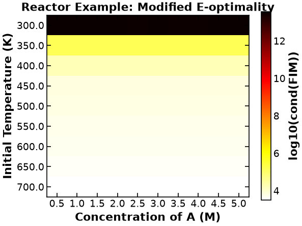
As an example, the reactor-case D-optimality figure shows:

The most informative region is around $C_{A0}=5.0 \ \text{M},$ $T=500.0 \ \text{K}$ . The least informative region is around $C_{A0}=0.5 \ \text{M},$ $T=300.0 \ \text{K}$ .

This can be a lot to take in at once, but think of each square within each plot as a unique experiment. To know what the optimality values are for an experiment set at an initial A concentration of 2.5 M and a temperature of 700 K, merely requires finding that location on the plots.

The power of viewing multiple experiments at once is that it gives a more contextualized view of the design space. Viewing one value is also possible, but it tells less of a complete story out of the surrounding space’s context.

Step 8: Compute D-Optimal Experiment Design (Optimization)¶

Computational Optimization¶

# Keep solver output compact for the course website.
doe_obj.tee = False

# Notice we specified the "determinant" objective when creating the DesignOfExperiments object
doe_obj.run_doe()

Extract and Summarize FIM¶

Next, we can summarize the FIM.

def results_summary(result):
    """Summarize the results of the experiment design
    Arguments:
    ----------
    result: The FIM matrix from the optimized experiment

    Returns:
    --------
    None

    Note: Taken from https://github.com/dowlinglab/pyomo-doe/blob/main/notebooks/tclab_pyomo.py

    """
    # The FIM is symmetric, so use eigh: it guarantees real eigenvalues in
    # ascending order, whereas the general-purpose eig returns a complex dtype.
    eigenvalues, eigenvectors = np.linalg.eigh(result)

    min_eig = min(eigenvalues)

    print("======Results Summary======")
    print("Four design criteria log10() value:")
    # NOTE: trace(FIM) is PSEUDO-A-optimality, not A-optimality.
    # A-optimality is min trace(FIM^-1). See Laky et al., Digital Discovery (2026),
    # Table 1, eqns (12) and (18).
    print("Pseudo-A-optimality:", np.log10(np.trace(result)))
    print("D-optimality:", np.log10(np.linalg.det(result)))
    print("E-optimality:", np.log10(min_eig))
    print("Modified E-optimality:", np.log10(np.linalg.cond(result)))
    print("\nFIM:\n", np.array(result))

    print("\neigenvalues:\n", eigenvalues)

    print("\neigenvectors:\n", eigenvectors)


results_summary(doe_obj.results["FIM"])

======Results Summary======
Four design criteria log10() value:
Pseudo-A-optimality: 6.931622012855398
D-optimality: 19.340418936129897
E-optimality: 3.138899447499543
Modified E-optimality: 3.7414680024488125

FIM:
 [[  177727.68204945    99344.01897622  -413450.1918958   -501980.23944408]
 [   99344.01897622   292559.39260089  -199013.3355907  -1435230.80982176]
 [ -413450.1918958   -199013.3355907    975776.53121599  1008827.37867208]
 [ -501980.23944408 -1435230.80982176  1008827.37867208  7097164.7083167 ]]

eigenvalues:
 [1.37689064e+03 2.21105032e+03 9.47443698e+05 7.59219668e+06]

eigenvectors:
 [[-0.91723826 -0.1168231  -0.37301041 -0.07674359]
 [-0.12385491  0.97210408  0.04024278 -0.1950747 ]
 [-0.37684436 -0.05406713  0.91113443  0.15779456]
 [-0.03636312  0.19606826 -0.17052213  0.96496485]]

Extract and Visualize Optimal Dynamic Experiment¶

Plot the optimized concentration and temperature trajectories. Use the plot to check bounds, continuity, and whether the selected profile is physically interpretable.

def plot_experiment_results(model):
    """
    Plot the results of the experiment design

    Arguments:
    ----------
    model: The Pyomo model

    Returns:
    --------
    None
    """
    # Extract the timepoints
    time = np.array([pyo.value(t) for t in model.t])

    # Extract the concentrations
    CA = np.array([pyo.value(model.CA[t]) for t in model.t])
    CB = np.array([pyo.value(model.CB[t]) for t in model.t])
    CC = np.array([pyo.value(model.CC[t]) for t in model.t])
    T = np.array([pyo.value(model.T[t]) for t in model.t])

    # Create the plot
    fig, ax1 = plt.subplots()

    # Plot concentrations on the left y-axis
    # Okabe-Ito colours paired with distinct linestyles (see figures/README.md):
    # blue/green/purple alone collapse to nearly the same grey in print.
    ax1.plot(time, CA, label="$C_A$", color="black", linestyle="-")
    ax1.plot(time, CB, label="$C_B$", color="#0072B2", linestyle="--")
    ax1.plot(time, CC, label="$C_C$", color="#E69F00", linestyle="-.")
    ax1.set_xlabel("Time (h)")
    ax1.set_ylabel("Concentration (mol/L)")
    ax1.legend(loc="upper left")

    # Create a second y-axis for temperature
    ax2 = ax1.twinx()
    ax2.plot(time, T, label="$T$", color="#D55E00", linestyle=":")
    ax2.set_ylabel("Temperature (K)", color="#D55E00")
    ax2.tick_params(axis="y", labelcolor="#D55E00")

    # Add legend for the temperature line
    ax2.legend(loc="upper right")

    plt.title("Experiment Results")
    plt.show()


# Plot the results of the experiment design
plot_experiment_results(doe_obj.model.scenario_blocks[0])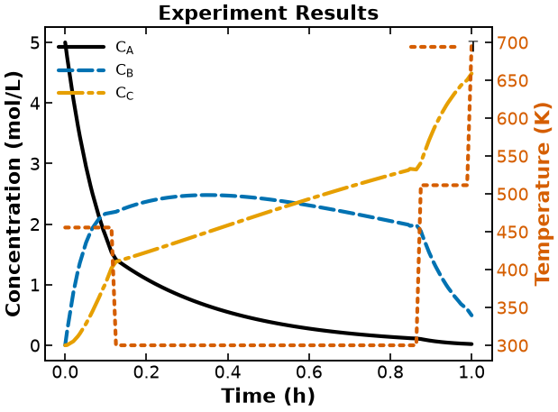

Key Takeaways¶

DOE is helpful for guiding decision-making by maximizing information yield in experimental design.
FIM allows us to gain information about the data from a mathematical model in an experiment.
Optimality conditions tell us the most and least informative regions in regards to the measurements in experimental design.
Heatmaps enable us to visualize the most informative parameters using the optimality conditions.