Stochastic Programming

This notebook was prepared by Jialu Wang and revised by Maddie Watson at the University of Notre Dame.

Farmer’s example: one model, reused¶

Read the physical balances, connect them to Pyomo Blocks, and analyze complete solution tables. The SAA, CVaR, and zero-VSS pages reuse this implementation. Further examples retain the optional uniform-yield, dependence, and profit-floor studies.

Textbook data: Birge and Louveaux (2011), 2nd ed., §1.1a–c, pp. 4–11.

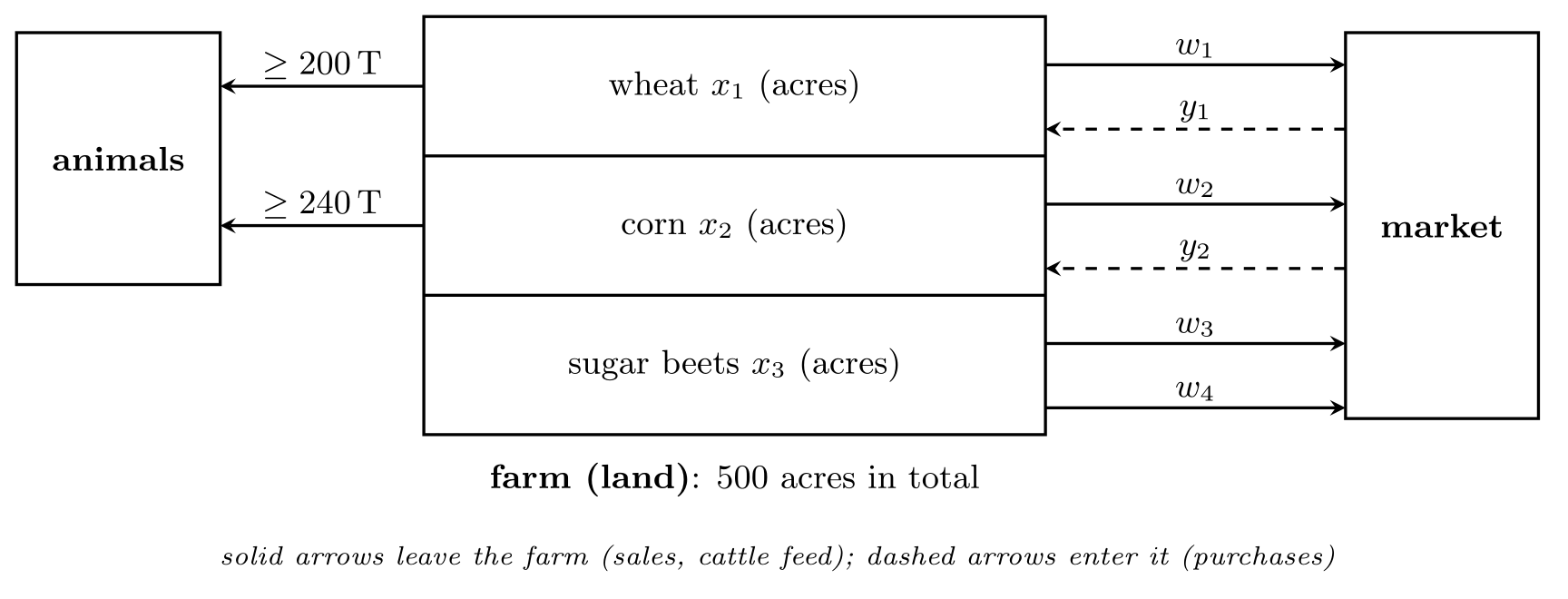
The textbook farmer example in Birge and Louveaux (2011), 2nd ed., §1.1a–c, pp. 4–11, uses 500 acres and three crops. Wheat and corn must supply 200 and 240 tons of feed; shortages can be purchased and surplus sold. Sugar beets have a premium-price sales cap of 6000 tons.

Total available land: 500 acres

To help the farmer make up his mind, we can set up the following model. Let

• $x_1$ = acres of land devoted to wheat,

• $x_2$ = acres of land devoted to corn,

• $x_3$ = acres of land devoted to sugar beets,

• $w_1$ = tons of wheat sold,

• $y_1$ = tons of wheat purchased,

• $w_2$ = tons of corn sold,

• $y_2$ = tons of corn purchased,

• $w_3$ = tons of sugar beets sold at the favorable price,

• $w_4$ = tons of sugar beets sold at the unfavorable price.

Deterministic mean-yield model¶

First solve at the specified mean yields. Later, the same model is solved separately at each realized yield to compute the perfect-information benchmark:

With $b$ tons available to sell, optimal beet revenue is $36\min(b,6000)+10\max(b-6000,0)$. The separate sales variables and premium bound represent this concave piecewise-linear revenue within an LP; binary variables are unnecessary for these prices.

Declare shared decisions and scenario Blocks¶

A Block groups variables, constraints, and expressions. The root model owns acreage; each scenario Block owns purchases and sales and refers to the same acreage variables. One scenario gives the deterministic LP. More scenarios reuse the model without copying planting decisions.

The builder and its helpers below are defined before the first solve. Monetary objectives use profit maximization; this is equivalent to minimizing net cost in the mathematical formulation above. Units are checked on the small models.

Shared helpers for the companion pages¶

The optional risk interface and complete-solution utilities below are also exported from this notebook. The introductory stochastic-programming model uses the default expected-profit objective; CVaR explains the risk formulation.

Known yields: solve, then interpret¶

build_farmer([correlated_scenario(1.0)]) creates the mean-yield LP. The same function receives a singleton list for each known-yield benchmark below.

Discuss: classify the problem. Why does the solution grow 300 acres of beets? Which resource limits the profit? The dual values report the local change in optimal profit per extra unit of the corresponding constraint bound.

The mean-yield model is an LP. Premium beet acreage reaches the sales quota; corn meets feed needs, and wheat takes the remaining land. The land multiplier is a local sensitivity, not a universal crop ranking. Crop rotation and shared labor constraints can change the allocation.

What if yields are known before planting?¶

Solve three separate problems: all crops at 120%, 100%, or 80% of mean yield. This assumes perfect information before planting.

Analyze the results: why does lower beet yield lead to more beet acreage? Why does the bad-year solution buy corn? Which assumption makes these three planting plans unavailable to a farmer who must plant before observing yields?

One planting plan, three possible harvests¶

• Stage 1: choose acreage before yield information.

• Stage 2: buy and sell after observing the harvest.

• Nonanticipativity: decisions use only information available at that time. One shared m.acreage enforces this structurally.

Each scenario has probability 1/3. The same build_farmer(THREE) function now creates three Blocks and maximizes expected profit.

Birge and Louveaux, §1.1b–c, pp. 6–11; §1.2, pp. 21, 25–26.

Stages describe information¶

A stage groups decisions that have the same information available. It need not be a fixed number of days. In this two-stage model the order is

The first-stage vector $\mathbf{x}$ is chosen before the uncertain yields are observed. Recourse $\mathbf{y}_s$ is chosen afterward, subject to the acreage already planted. Planning for recourse means accounting for those future feasible actions when choosing $\mathbf{x}$ today. It does not mean waiting to choose every variable until the harvest is known.

Nonanticipativity requires identical decisions whenever scenarios have identical information histories at the decision time. All three farmer scenarios have the same history at planting, so they share acreage. After the harvest is observed, their trading decisions may differ. In a multistage tree, decisions remain shared at a common node and can separate only after the histories branch. See Birge and Louveaux, §1.2, pp. 21, 25–26, and §§2.3–2.4, pp. 57–60.

Random vectors, realizations, and scenarios¶

$\boldsymbol{\Xi}$ denotes a random vector of uncertain data; $\boldsymbol{\xi}$ is one realized value. The joint law specifies which combinations occur and with what probabilities. Its support $\Theta\subseteq\mathbb{R}^d$ is the smallest closed set with probability one. The book writes $\Xi$ for this support; here uppercase bold $\boldsymbol{\Xi}$ identifies the random vector. We use $\Omega$ for the finite retained scenario indices below, whereas the book also uses $\Omega$ for an underlying sample space.

For a finite distribution, scenario $s\in\Omega$ has realization $\boldsymbol{\xi}_s$ and probability $p_s>0$, with $\sum_s p_s=1$. Zero-probability scenarios may be removed. A fair die has six outcomes, each of probability $1/6$. For an event $A$,

A probability density $p_{\boldsymbol{\Xi}}$ instead satisfies

A density value is not a probability at a point and can exceed one. For example, $U\sim\operatorname{Uniform}(0,1/2)$ has density 2 on that interval, total area $2(1/2)=1$, and $\Pr(0\le U\le1/4)=2(1/4)=1/2$; each individual point has probability zero.

For an integrable function $\phi$,

The weighted sum is exact when it includes the full finite law. A retained sample of a continuous law gives a discrete approximation; independent identically distributed sampling uses empirical weights $1/N$. The mean and covariance summarize a law but do not specify it. Likewise, independent draws across scenarios do not imply independent crops within a scenario: shared weather can correlate all three crop yields. The SAA guide supplies a declared joint generator and its complete 20-row sample. See Birge and Louveaux, §§2.1–2.2, pp. 55–57, and §1.1d, pp. 11–15.

General two-stage model and extensive form¶

A general finite-scenario net-cost minimization model is

Here $\mathbf{x}\in\mathbb{R}^{n_1}$ is shared, $\mathbf{y}_s\in\mathbb{R}^{n_2}$ is scenario-specific, and $X,Y_s$ include variable domains. Every positive-probability scenario has its own feasibility constraints; the probability weights do not relax those constraints. This $f,\mathbf{g},\mathbf{h}$ form allows nonlinear functions or integer domains. The expanded farmer model below is an LP because its coefficients are fixed once a scenario is specified and every variable is continuous.

The book’s classical linear fixed-recourse form makes the nested optimization explicit:

$W$ is the recourse matrix, common to scenarios; “fixed recourse” does not require fixed recourse decisions. The data $\mathbf{q}_s,\mathbf{h}_s,T_s$ may depend on the realization. For a continuous law, recourse constraints hold almost surely, meaning outside a set of probability zero. For a retained finite law, each positive-probability row must be feasible. For a given $\mathbf{x}$, infeasible recourse has value $+\infty$ in the net-cost convention. An expected-cost model also needs a well-defined finite expectation at the policies being compared.

Substitute the full finite law into the expectation and include each scenario’s recourse variables:

This extensive form optimizes one planting decision and all contingent trading decisions together. It is equivalent to the nested recourse formulation when the finite scenario law is exact and the recourse optima exist. If a first-stage cost is included inside every $f_s$, then $\sum_s p_s\mathbf{c}^{\mathsf T}\mathbf{x}=\mathbf{c}^{\mathsf T}\mathbf{x}$; it is counted once because weights sum to one.

An alternative implementation creates a copy $\mathbf{x}_s$ per scenario and adds

Any feasible shared-vector solution gives feasible copies by setting each copy to $\mathbf{x}$. Conversely, these equalities force every feasible copied solution to use that same vector, giving the same scenario constraints and objective. Thus the formulations are equivalent. Removing the equalities instead permits perfect-information planting and changes the information structure. build_farmer avoids the extra copies by referring to the root acreage in every Block. See Birge and Louveaux, §1.2, model (2.2), pp. 25–26; §2.4, pp. 59–60; and §3.1a, pp. 103–104.

Preserve dependence within a scenario¶

Both constructed laws give each crop a normalized yield of 0.8 or 1.2 with equal probability and mean one. Under common weather, both low yields occur with probability one half; under independence, with probability one quarter. Thus the means and marginals do not determine the joint law. The joint profit distribution and its tail can change. For this farmer’s additive, crop-separable expected recourse, holding all crop marginals fixed leaves the population risk-neutral objective unchanged; the full separability argument explains the required structure. Finite sampled marginals may still differ across runs.

Analyze the results: compare acreage with the three perfect-information plans. Explain the switch between buying and selling corn. Does maximizing expected profit protect the worst-year outcome?

The extensive form has 3 shared acreage variables and 6 trading variables per scenario: 21 variables total. With the quota as a bound, there are 10 explicit inequalities (one land limit and three balances per scenario), plus variable bounds. None is an equality; subtracting inequality counts is not a degrees-of- freedom calculation.

In the figure, each $T_s$ is the scenario coefficient block multiplying shared acreage and $W_s$ multiplies that scenario’s trades. Quota bounds are omitted from the block sketch. Shaded blocks may include zero coefficients; the empty off-diagonal blocks are all zero.

Compare information values consistently¶

Use profit maximization throughout this comparison. Let $F(\mathbf{x},\boldsymbol\xi)$ include optimal trading after yields are observed.

Values are rounded after averaging; Birge and Louveaux, §4.1, pp. 163–164.

Expected value of perfect information¶

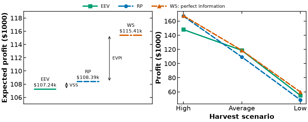
For profit maximization, $EVPI=WS-RP\approx\$7,015.56$. It is the model’s increase in optimal expected profit if yields are known before planting. It bounds a risk-neutral decision maker’s willingness to pay for perfect yield information within this model, not the price of an arbitrary forecast. See Birge and Louveaux, §4.1, pp. 163–164.

Expected-value plan evaluated under uncertainty¶

Choose $\bar{\mathbf{x}}\in\arg\max_{\mathbf{x}}F(\mathbf{x},\mathbb E[\boldsymbol\Xi])$ and then compute $EEV=\mathbb E[F(\bar{\mathbf{x}},\boldsymbol\Xi)]$. Only acreage is fixed; trading is optimized per scenario.

For the mean-yield plan (120,80,300), $EEV=\$107,240$. See Birge and Louveaux, §4.2, p. 165.

Value of the stochastic solution¶

With the profit convention, $VSS=RP-EEV=\$108,390-\$107,240=\$1,150$. The general ordering $WS\ge RP\ge EEV$ assumes a feasible EV plan and consistently optimized recourse. See Birge and Louveaux, §§4.2–4.3, pp. 165–166.

Why the information values have this order¶

Assume the optima below exist, their expected profits are finite, and the expected-value acreage $\bar{\mathbf{x}}$ admits feasible recourse in every retained scenario. Let $X$ impose the first-stage restrictions and let $F(\mathbf{x},\boldsymbol{\xi}_s)$ be the maximum scenario profit after optimizing trades at that fixed acreage. Acreage infeasible for a scenario can be excluded from that scenario’s maximization. Write $\mathbf{x}^*$ for an optimal shared plan and $\mathbf{x}^{WS}_s$ for a scenario’s perfect-information plan.

1. For each scenario, $\mathbf{x}^*$ is an available candidate when planting may use perfect information. Therefore

   $$F(\mathbf{x}^{WS}_s,\boldsymbol{\xi}_s)\ge F(\mathbf{x}^*,\boldsymbol{\xi}_s).$$

   (12)

   Multiply by $p_s\ge0$ and sum: $WS\ge RP$.

2. The shared stochastic optimum can choose the feasible candidate $\bar{\mathbf{x}}$, so

   $$RP=\max_{\mathbf{x}}\sum_s p_sF(\mathbf{x},\boldsymbol{\xi}_s) \ge\sum_s p_sF(\bar{\mathbf{x}},\boldsymbol{\xi}_s)=EEV.$$

   (13)

Consequently $WS\ge RP\ge EEV$, $EVPI=WS-RP\ge0$, and $VSS=RP-EEV\ge0$. The first inequality relaxes a restriction on information; the second compares an optimized plan with one feasible candidate. Neither proof requires convexity. For net-cost minimization every profit changes sign, giving $WS\le RP\le EEV$, $EVPI=RP-WS$, and $VSS=EEV-RP$. This is the profit-form derivation of Birge and Louveaux, §4.3, Proposition 1, p. 166.

Scope. If the mean-data plan is infeasible in a retained scenario, a finite EEV cannot be assumed; one must report infeasibility or explicitly introduce and price emergency recourse. A feasible plan’s trades must be reoptimized for each harvest. Reusing mean-harvest trades is a different, more restricted policy. The mean-data optimum $EV$ is also a different quantity from the expected realized profit $EEV$: here $EV=\$118,600$, while $EEV=\$107,240$.

There is no general ordering between EVPI and VSS. The alternative-price farmer gives a fully solved case with zero VSS and positive EVPI; Birge and Louveaux, §4.4, pp. 167–170, also treats the reverse case. EVPI concerns perfect information before the decision. VSS concerns optimizing the given probability law rather than its mean-data replacement. It is not the value of learning that law.

For risk-neutral expected profit, a forecast that only supplies partial yield information and leaves this model’s actions, prices, and uncertainty law unchanged cannot improve expected profit by more than perfect information does. An $8,000 forecast therefore cannot cover its cost when $EVPI\approx\$7,015.56$. This comparison does not price additional benefits outside the stated model.

The square, diagonal, and fixed point illustrate the feasible-set argument. The drawing normalizes one decision to $[0,1]$ and omits other constraints; it does not assert that the full farmer feasible set is a square.

EVPI measures the value of perfect pre-decision information. VSS compares the stochastic optimum with the evaluated mean-data plan; it does not measure the value of learning an unknown distribution.

Reference vocabulary and notation¶

These definitions use profit maximization. The CVaR guide, SAA guide, and advanced sampling study develop their respective formulations and computations.

Core stage, probability, and information-value definitions follow Birge and Louveaux, §§2.1–2.4, pp. 55–60, and §§4.1–4.3, pp. 163–166. General-distribution VaR/CVaR definitions follow Rockafellar and Uryasev (2002), Definitions 1 and 3 and Proposition 8; see the primary source links. The SAA guide cites Mak, Morton and Wood (1999) and Bayraksan and Morton (2006).

Complete solutions: acreage and all trades¶

Every purchase and sale quantity below is in metric tons. Profit includes planting cost. Perfect-information solutions choose a different acreage vector for each known harvest; the recourse and expected-value policies each plant once.

These are the full solutions used in the lecture handouts. The expected-value policy is evaluated with new optimal trades in each scenario, rather than reusing trades computed at mean yields.

Applications: identify what can adapt¶

For every model, specify the decision, the uncertain information, and which decisions remain available afterward. The stages follow that information structure. They do not follow whether a variable happens to appear in a scenario Block.

One robot for many tasks¶

Bravo-Palacios, Del Prete, and Wensing (2020) optimize a shared robot morphology together with scenario-specific trajectories. The physical design $\boldsymbol\rho$ includes quantities such as limb dimensions and actuator gear ratios. A scenario describes the task or environment; its state and control trajectories $\mathbf{x}_s(t),\mathbf{u}_s(t)$ may adapt to it. Their multiple-task formulation has the structure

subject to each scenario’s dynamics, path constraints, and boundary conditions, with one shared design. The paper uses direct collocation to transcribe the trajectory problems into an NLP. Its planar-manipulator and hopping-robot cases therefore connect the course’s dynamic optimization and stochastic modeling topics; they are not farmer LPs. A high probability weight does not make an infeasible design feasible in another required scenario.

Course connection, reported by Prof. Dowling: this work grew out of a Notre Dame student taking an early offering of this course. That teaching history is instructor-supplied context, separate from the paper’s claims.

Source: Bravo-Palacios, Del Prete & Wensing (2020), pp. 1680–1682, Fig. 1 and §II.A, Eq. (6).

Port capacity before freight demand¶

Bhurtyal et al. (2024) choose integer investments in loading equipment and storage facilities under a budget. After freight demand is realized, transportation and inventory decisions adapt within the installed capacity. The objective combines investment cost with expected transportation cost. The modeled network includes ports, supply/demand regions, truck and rail links, and barge movement.

The farmer analogy is capacity rather than crop identity: installed equipment and storage correspond to shared acreage; scenario-specific flows correspond to recourse trades. Integer investment variables distinguish this model from the continuous farmer LP. The source’s reported economic effects belong to its case data and are not generic benefits guaranteed by stochastic optimization.

Source: Bhurtyal et al. (2024), §3, pp. 190–191, Eqs. (1)–(5).

Mitigate now, restore after a flood¶

Zhang and Alipour (2023) choose pre-event bridge mitigation and construction actions, then scenario-specific restoration resources and techniques after weather-related damage. Traffic assignment represents network use during construction and recovery. Their formulation combines investment and disruption consequences with expected post-event costs and contains integer decisions and nonlinear network behavior.

The two-stage restriction keeps the mitigation choice common across flood scenarios. Recovery may vary because damage is then observed. Calling this second-stage action recourse distinguishes it from a WS benchmark, which would also allow the earlier mitigation decision to use perfect information. User-equilibrium traffic assignment should not be interpreted as a general guarantee of minimum total system travel time.

Source: Zhang & Alipour (2023), §3.3, pp. 416–417, first-stage formulation (1)–(15) and recourse formulation (16)–(27).

CO₂ transport investment as capacity changes¶

Zhang, Anjos, and Chalmers (2026) plan pipeline and ship infrastructure while future capture capacity may expand, close, or reactivate. Decisions adapt over several information stages. At a common scenario-tree node, scenarios with the same observed history share the investment decision; a model that allowed a different early investment for each full future path would anticipate information.

The Humber-cluster study uses a 40-year horizon with seven stages, including a final operating stage without new construction. Those are case assumptions. The general lesson is the evolving information structure and the cost of committing capacity before demand for transport is resolved. A two-stage simplification would need to state when the remaining uncertainty becomes known and which subsequent choices it allows.

Source: Zhang, Anjos & Chalmers (2026), §§2.1–2.2, physical PDF pp. 5–6 and Fig. 1; article 11, rather than an eleven-page range.

Process systems: match the model to the uncertainty¶

Li and Grossmann’s 2021 review surveys stochastic programming for process design, planning, scheduling, and control. Table 1 pairs applications with uncertain quantities, including supply, prices, feed composition, demand, yields, and technology or clinical outcomes. These are entry points for choosing a modeling structure; a common vocabulary does not make their feasible sets or information assumptions interchangeable.

For a process-design application, identify installed equipment and sizing decisions, then identify the operating actions available after uncertain feeds or demands are observed. A scheduling application may instead place decisions at several release times. Risk-neutral expected cost, tail-risk criteria, chance constraints, and robust requirements answer different questions.

Source: Li & Grossmann (2021), §1 and Table 1, pp. 2–3. Its literature counts describe the review’s historical search window, not a current field census.

For another complete formulation and executable Block example, see A Small Two-Stage Production Plan. It is optional reading; the farmer remains the common example of the two lecture handouts.

Probability of compliance and further directions¶

For a specified probability law $\mathbb P$ and allowed violation probability $0\le\varepsilon<1$, a chance constraint requires

A joint chance constraint instead protects all listed requirements together:

Separate bounds $\Pr(g_j\le0)\ge1-\varepsilon_j$ imply only the union-bound guarantee $\Pr(g_j\le0\ \forall j)\ge1-\sum_j\varepsilon_j$, without further assumptions. For example, among 20 equal-probability outcomes, let only outcome 1 violate A and only outcome 2 violate B. Each requirement holds with probability 0.95; both hold together with probability 0.90. Independence is not assumed in this construction.

Chance constraints limit violation probability under the declared law. CVaR instead measures the severity of unfavorable outcomes in a chosen tail. Neither criterion corrects an incorrectly specified probability law. In an empirical chance constraint, meeting the retained sample requirement is also different from certifying population reliability. See Pagnoncelli, Ahmed & Shapiro (2009), §1, Eq. (1), p. 400 and §2, for the sampled formulation and its theory.

Application and theory entry points¶

• Process optimization: Li, Arellano-Garcia & Wozny (2008), §§2–3, uses probability requirements for uncertain operating quantities. State whether one requirement or simultaneous compliance is protected.

• Assistive-robot activities: Bevilacqua et al. (2021), §III, p. 3953, concerns activity/point-of-interest selection with probabilistic resource limits. This is not a general guarantee of low-level physical safety.

• Sampling: Pagnoncelli et al., §§2–4, develops SAA theory with portfolio and blending applications. Sampling error and the chosen violation probability are separate quantities.

Information can arrive repeatedly or depend on decisions¶

Multistage programming adapts decisions as information arrives. Scenarios sharing the observed history must share decisions at that node. Ding, Hu & Bie (2018), §II, pp. 319 onward, applies nonanticipativity to joint power and natural-gas expansion. The CO₂ transport case is another multistage example. A full-path scenario index alone does not enforce the correct information restriction.

Decision-dependent uncertainty permits decisions to alter the probability law, the information available later, or both. Yin & Hou (2024), §2, reviews these distinctions in power systems. The farmer’s exogenous yield generator does not model either effect: planting changes harvest quantity at a realized yield, rather than changing the yield distribution.

Distributionally robust chance constraints require probability compliance across an ambiguity set $\mathcal P$ of candidate laws, for example

Jiang & Guan (2016), §1.2, pp. 294–295 and §3, Theorem 1, p. 298, studies a particular $\phi$-divergence ambiguity set. Its reformulation should not be generalized to arbitrary ambiguity sets. Ambiguity about a law differs from variation of outcomes under one known law.

For alternative risk measures and a complete fixed-production case, see Risk Measures and Portfolio Optimization. For replicated optimality-gap estimation and quadrature detail, see Advanced Topics in Stochastic Programming. Those pages supplement the handouts; their assumptions and sign conventions must be carried into any comparison.