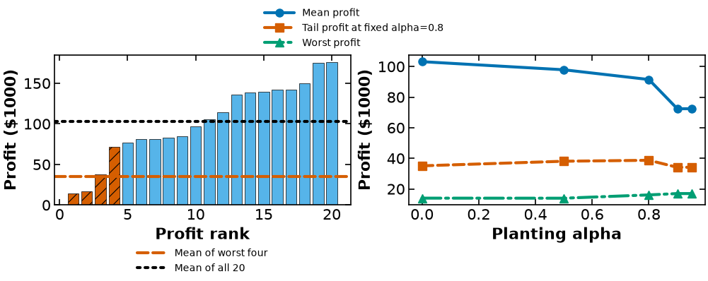
Use the same 20 synthetic harvests to examine the price of protecting bad outcomes. First inspect a fixed plan’s profit distribution, then optimize the planting decision. All distributions below are finite empirical distributions with equal weights.
import sys
from pathlib import Path
if "google.colab" in sys.modules:
    from urllib.request import urlretrieve
    base = "https://raw.githubusercontent.com/ndcbe/optimization/main/notebooks/"
    for name in ["helper.py", "farmer.py"]:
        urlretrieve(base + name, name)
    import helper
    helper.easy_install()
else:
    sys.path.insert(0, str(Path.cwd().parent))
    import helper
import farmer as f
import numpy as np
import pandas as pd
import matplotlib.pyplot as plt
from IPython.display import display
helper.set_plotting_style()
def show_solution(record):
    display(pd.Series(record["acreage"], name="Planted acres").to_frame().round(3))
    rows = []
    for s in record["scenarios"]:
        row = {"Scenario": s["id"], "Probability": s["probability"]}
        row.update({"Buy " + c + " (T)": v for c, v in s["purchases_tons"].items()})
        row.update({"Sell " + c + " (T)": v for c, v in s["sales_tons"].items()})
        row["Profit ($)"] = s["profit"]
        rows.append(row)
    display(pd.DataFrame(rows).set_index("Scenario").round(2))
    print(f"Expected profit: ${record['expected_profit']:,.2f}")
Loss, quantile, and tail average
Write loss as . At confidence level , VaR is the smallest threshold with cumulative probability at least . CVaR averages the worst probability mass , including only the required fraction of an atom at the cutoff.
For 20 equal weights and , that tail is the four worst outcomes. A loss can be negative: positive profit corresponds to negative loss. We display the equivalent lower-tail profit , so larger is better.
neutral = f.solve_farmer(f.build_farmer(f.TWENTY))
neutral_record = f.evaluate_solution(f.plan_of(neutral), f.TWENTY)
profits = np.array([s["profit"] for s in neutral_record["scenarios"]])
order = np.argsort(profits)
display(pd.DataFrame({"Scenario": order+1, "Profit ($)": profits[order]}).round(2))
print("Mean profit:", profits.mean())
print("Lower-tail profit at alpha=0.8:", f.lower_tail_profit(profits, .8))
Mean profit: 103193.43152366493
Lower-tail profit at alpha=0.8: 35109.66974272152
The optimization problem and Pyomo
Retain the farmer land, feed, beet-quota, and nonnegativity constraints. Add
This is an epigraph formulation: auxiliary variables bound the positive-part losses from above. In profit notation, gives the equivalent maximization below. The crop balances and shared acreage are unchanged.
def attach_tail_objective(m, alpha):
    """Maximize the lower-tail profit: equivalent to minimizing CVaR of loss."""
    if not 0 <= alpha < 1:
        raise ValueError("Use 0 <= alpha < 1")
    m.nu = f.pyo.Var(units=f.u.USD)
    m.z = f.pyo.Var(m.SCENARIOS, domain=f.pyo.NonNegativeReals, units=f.u.USD)
    m.tail_shortfall = f.pyo.Constraint(
        m.SCENARIOS, rule=lambda m, s: m.z[s] >= m.nu - m.scenarios[s].profit)
    m.objective.deactivate()
    m.tail_objective = f.pyo.Objective(
        expr=m.nu-sum(m.weight[s]*m.z[s] for s in m.SCENARIOS)/(1-alpha),
        sense=f.pyo.maximize)
policies = []
for alpha in [0, .5, .8, .9, .95]:
    m = f.build_farmer(f.TWENTY)
    attach_tail_objective(m, alpha)
    f.solve_farmer(m)
    record = f.evaluate_solution(f.plan_of(m), f.TWENTY)
    p = np.array([s["profit"] for s in record["scenarios"]])
    np.testing.assert_allclose(p, f.analytic_profits(f.plan_of(m), f.TWENTY), atol=1e-6)
    np.testing.assert_allclose(f.pyo.value(m.tail_objective),
                               f.lower_tail_profit(p, alpha), atol=1e-6)
    policies.append({"alpha": alpha, "solution": record,
                     "optimized_tail": f.lower_tail_profit(p, alpha),
                     "common_tail80": f.lower_tail_profit(p,.8), "worst": float(p.min())})
display(pd.DataFrame([{"alpha": r["alpha"], **r["solution"]["acreage"],
    "Mean profit": r["solution"]["expected_profit"], "Tail at own alpha": r["optimized_tail"],
    "Tail at fixed alpha=.8": r["common_tail80"], "Worst": r["worst"]}
    for r in policies]).round(2))
Complete solution for a representative risk-averse policy
The alpha = 0.8 plan protects the worst four outcomes in this scenario model. Compare its land allocation and every recourse quantity with the risk-neutral solution. No claim is made that this is the right risk preference for every farmer.
show_solution(policies[2]["solution"])
Expected profit: $91,519.31
results = {"neutral": neutral_record, "policies": policies,
           "inputs20": [s["yield"] for s in f.TWENTY]}
helper.save_results("farmer-cvar-twenty", results,
    notebook="notebooks/4-dev/Farmer_CVaR.ipynb", source_tag="handout:farmer-tail-objective",
    solver="appsi_highs", description="Complete recourse and CVaR policies for 20 synthetic harvests",
    source_files=["notebooks/farmer.py"],
    source_cells=[("notebooks/4-dev/Farmer_CVaR.ipynb", "provenance:farmer-cvar-policy-study")])
[helper] wrote figures/results/farmer-cvar-twenty.json
p = np.array([s["profit"] for s in results["neutral"]["scenarios"]])
order = np.argsort(p)
fig, axes = plt.subplots(1, 2, figsize=(10, 4), layout="constrained")
for j, i in enumerate(order):
    axes[0].bar(j+1, p[i]/1000, color="#D55E00" if j<4 else "#56B4E9",
                hatch="//" if j<4 else "", edgecolor="black", linewidth=.5)
axes[0].axhline(p[order[:4]].mean()/1000, color="#D55E00", ls="--",
               label="Mean of worst four")
axes[0].axhline(p.mean()/1000, color="black", ls=":", label="Mean of all 20")
axes[0].set(xlabel="Profit rank", ylabel="Profit ($1000)")
rows=results["policies"]; alpha=[r["alpha"] for r in rows]
for key, label, color, marker in [("mean", "Mean profit", "#0072B2", "o"),
    ("common_tail80", "Tail profit at fixed alpha=0.8", "#D55E00", "s"),
    ("worst", "Worst profit", "#009E73", "^")]:
    vals=[r["solution"]["expected_profit"] if key=="mean" else r[key] for r in rows]
    axes[1].plot(alpha, np.array(vals)/1000, color=color, marker=marker, label=label)
axes[1].set(xlabel="Planting alpha", ylabel="Profit ($1000)")
fig.legend(*axes[1].get_legend_handles_labels(), loc="outside upper center", ncol=1, fontsize=10)
axes[0].legend(loc="upper center", bbox_to_anchor=(.5,-.23), fontsize=10)
helper.save_figure(fig, "farmer-cvar-twenty")
[helper] wrote media/figures/farmer-cvar-twenty.png and .pdf
Endpoints and implementation detail
At alpha = 0, the entire distribution is in the tail, so the objective is expected profit. With 20 equal weights, alpha at least 0.95 and below 1 selects only the worst outcome. This is a worst-case criterion for the retained scenarios, not every possible harvest. Do not substitute alpha = 1 into the formula.
The optimized threshold need not be unique, especially at discrete quantiles. Calculate reported CVaR from the resulting distribution, including partial atom mass, rather than treating an arbitrary solver threshold as a unique statistical estimate.
A pure tail objective need not reward efficient trades in a good scenario. We therefore fix optimized acreage and maximize profit separately in every scenario before reporting the policy’s outcomes. This improves recourse without altering planting decisions. The independent piecewise recourse formula checks every reported profit.
For a mean/tail blend, maximize at fixed alpha. Alpha selects tail probability; lambda weights the two criteria. Comparing policies using a common fixed-alpha metric avoids confusing a changed definition of the tail with a changed planting decision.
Primary sources: Rockafellar & Uryasev (2000), Optimization of Conditional Value-at-Risk, DOI; Rockafellar & Uryasev (2002), Conditional value-at-risk for general loss distributions, Definitions 1 and 3, Proposition 8, Theorem 10 and Corollary 12, DOI.
Balance mean profit and the same tail
At a fixed , maximize for . Here changes the importance of the unfavorable tail while its definition stays fixed. The table reports separately reoptimized recourse for each chosen acreage and evaluates every policy on the same 20 harvests. Compare the endpoints and explain the acreage shift; values between them need not change smoothly.
blend_rows = []
for weight in [0, .25, .5, .75, 1.0]:
    blend = f.solve_farmer(f.build_farmer(f.TWENTY, risk={"cvar": (.8, weight)}))
    solved = f.evaluate_solution(f.plan_of(blend), f.TWENTY)
    profits = np.array([s["profit"] for s in solved["scenarios"]])
    np.testing.assert_allclose(profits, f.analytic_profits(f.plan_of(blend), f.TWENTY), atol=1e-6)
    blend_rows.append({"Mean weight": 1-weight, "Tail weight": weight,
        **solved["acreage"], "Mean profit ($)": solved["expected_profit"],
        "CVaR profit at alpha=.8 ($)": f.lower_tail_profit(profits, .8),
        "Worst profit ($)": profits.min()})
display(pd.DataFrame(blend_rows).round(2))
How planting and production change with alpha
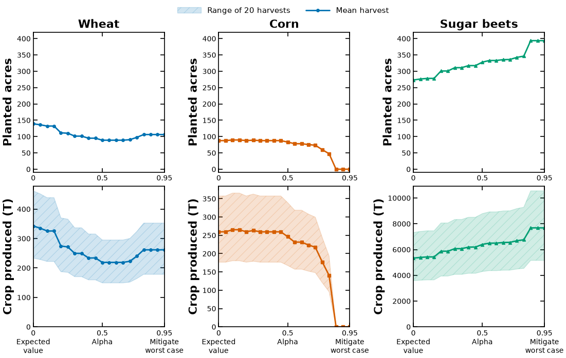
At alpha = 0, optimizing CVaR is expected-value optimization. At alpha = 0.95, the tail contains one of the 20 equally weighted scenarios, so the objective mitigates the worst case within this sample.
The top row shows planted acreage. The bottom row shows mean crop production and the full range across the same 20 harvests. Production means harvest before purchases or sales. Shading is a scenario range, not a confidence interval. Solutions are computed on a grid of alpha values; connecting lines guide the eye and do not imply a smoothly changing optimizer.
alpha_sweep = []
yields20 = np.array([[s["yield"][c] for c in f.CROPS] for s in f.TWENTY])
for alpha in np.linspace(0, .95, 20):
    m = f.build_farmer(f.TWENTY)
    attach_tail_objective(m, float(alpha))
    f.solve_farmer(m)
    acreage = f.plan_of(m)
    production = yields20 * acreage
    profits = f.analytic_profits(acreage, f.TWENTY)
    np.testing.assert_allclose(f.pyo.value(m.tail_objective),
                               f.lower_tail_profit(profits, alpha), atol=1e-6)
    alpha_sweep.append({"alpha": float(alpha), "acreage": acreage.tolist(),
        "production_mean": production.mean(axis=0).tolist(),
        "production_min": production.min(axis=0).tolist(),
        "production_max": production.max(axis=0).tolist(),
        "tail_profit": f.lower_tail_profit(profits, alpha)})
results = {"sweep": alpha_sweep, "yields20": yields20.tolist(),
           "crops": f.CROPS, "seed": f.SYNTHETIC_SEED}
helper.save_results("farmer-alpha-acreage-production", results,
    notebook="notebooks/4-dev/Farmer_CVaR.ipynb", source_tag="handout:farmer-tail-objective",
    solver="appsi_highs", description="Acreage and harvest production versus alpha; 20 equal-weight scenarios",
    source_files=["notebooks/farmer.py"],
    source_cells=[("notebooks/4-dev/Farmer_CVaR.ipynb", "provenance:farmer-alpha-sweep")])
[helper] wrote figures/results/farmer-alpha-acreage-production.json
rows = results["sweep"]
a = np.array([r["alpha"] for r in rows])
fig, axes = plt.subplots(2, 3, figsize=(11, 7), layout="constrained")
for j, (crop, color, marker) in enumerate(zip(
    ["Wheat", "Corn", "Sugar beets"], ["#0072B2", "#D55E00", "#009E73"], ["o", "s", "^"])):
    planted = np.array([r["acreage"][j] for r in rows])
    mean = np.array([r["production_mean"][j] for r in rows])
    low = np.array([r["production_min"][j] for r in rows])
    high = np.array([r["production_max"][j] for r in rows])
    axes[0,j].plot(a, planted, color=color, marker=marker, ms=4, linewidth=2)
    axes[0,j].set(title=crop, ylabel="Planted acres", ylim=(-10, 420))
    axes[1,j].fill_between(a, low, high, color=color, alpha=.18, hatch="//",
                           label="Range of 20 harvests")
    axes[1,j].plot(a, mean, color=color, marker=marker, ms=4, linewidth=2,
                   label="Mean harvest")
    axes[1,j].set(ylabel="Crop produced (T)")
    axes[1,j].set_ylim(bottom=0)
    for ax in axes[:,j]:
        ax.set_xlim(0,.95)
        ax.tick_params(labelsize=10)
    axes[0,j].set_xticks([0,.5,.95], labels=["0", "0.5", "0.95"])
    axes[1,j].set_xticks([0,.5,.95], labels=["0\nExpected\nvalue", "0.5\nAlpha", "0.95\nMitigate\nworst case"])
fig.legend(*axes[1,0].get_legend_handles_labels(), loc="outside upper center", ncol=2, fontsize=11)
helper.save_figure(fig, "farmer-alpha-acreage-production")
[helper] wrote media/figures/farmer-alpha-acreage-production.png and .pdf
- Rockafellar, R. T., & Uryasev, S. (2000). Optimization of conditional value-at-risk. The Journal of Risk, 2(3), 21–41. 10.21314/jor.2000.038
- Rockafellar, R. T., & Uryasev, S. (2002). Conditional value-at-risk for general loss distributions. Journal of Banking & Finance, 26(7), 1443–1471. 10.1016/s0378-4266(02)00271-6