This notebook contains material from cbe67701-uncertainty-quantification; content is available on Github.
8.1 First-Order Second-Moment (FOSM) Method Example
Zihan (Zora) Huang (zhuang2@nd.edu) July 6th, 2020
The follow text, example, and code were adapted from:
McClarren, Ryan G (2018). Uncertainty Quantification and Predictive Computational Science: A Foundation for Physical Scientists and Engineers, Chapter 8: Reliability Methods for Estimating the Probability of Failure, Springer, https://doi.org/10.1007/978-3-319-99525-0_8
8.1.1 Summary: Reliability Methods for Estimating the Probability of Failure
Reliability methods are a class of techniques that seek to answer the question of with what probability a QoI will cross some threshold value.
Reliability methods will try to characterize the safety of the system using a single number, $\beta$ (reliability of index), expressed as the number of standard deviations above the mean performance where the failure point of the system is.
Reliability methods try to estimate the system performance using a minimal number of QoI evaluations to infer system behavior, and endeavir that necessarily requires extrapolation from a few data points to an entire distrition.
Contrast to previous chapters about sampling, where actual samples from the distribution of the QoI was needed to make statements about a distribution, at a cost of requiring many evaluations of QoI. Fewer evaluations are required in reliability analysis, therefore faster.
Simplifications made reliability method less robust, therefore assumptions and approximations in such calculations needs to be clarified.
8.1.2 First-Order Second-Moment (FOSM)
The simplest and least expensive type of reliability method involves extending the sensitivity analysis we have already completed to make statments about the values of the distribution.
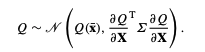
The first-order second-moment (FOSM) uses first-order sensitivities to estimate the variance. Using the assumption that the value of QoI at the mean of the inputs is the mean of the QoI:

An additional assumption is that the QoI is normal with a known mean and variance.
Using the covariance matrix of the inputs, along with the sensitivities,
$ \frac{dQ}{dx_i}$, to estimate the variance:

Q is normally distributed as:
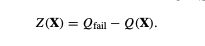
Reliability analysis typically rescales the QoI so that the point we are interested in, the so-called failure point, experessed in quantity, $Z$, such that failure occurs when $Z$ < 0. To use the failure value of QoI, $Q_fail$, to define $Z$:
The probability of failure is:
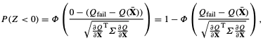
where $\phi(x)$ is the standard nomral CDF.
The probability of failure leads toi the defination of the reliability index for the system. The reliability index, $\beta$, is defined as:

Import Libraries and Download Figures
import matplotlib.pyplot as plt
from scipy.stats import norm
import numpy as np
import matplotlib.pyplot as plt
import scipy.stats as stats
%matplotlib inline
# Download figures (if needed)
import os, requests, urllib

# GitHub pages url
url = "https://ndcbe.github.io/cbe67701-uncertainty-quantification/"

# relative file paths to download
# this is the only line of code you need to change
file_paths = ['figures/Fig-8.1.7.png']

# loop over all files to download
for file_path in file_paths:
    print("Checking for",file_path)
    # split each file_path into a folder and filename
    stem, filename = os.path.split(file_path)

    # check if the folder name is not empty
    if stem:
        # check if the folder exists
        if not os.path.exists(stem):
            print("\tCreating folder",stem)
            # if the folder does not exist, create it
            os.mkdir(stem)
    # if the file does not exist, create it by downloading from GitHub pages
    if not os.path.isfile(file_path):
        file_url = urllib.parse.urljoin(url,
                urllib.request.pathname2url(file_path))
        print("\tDownloading",file_url)
        with open(file_path, 'wb') as f:
            f.write(requests.get(file_url).content)
    else:
        print("\tFile found!")
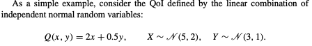
# Example 8.1: Fig.8.1 FOSM example of linear combination of independent normal random variables

x = np.linspace (-2,10,100)
mean_x = 5
sigma_x = 2
y = x
mean_y = 3
sigma_y = 1

# estimation of mean using EQN. 8.1

Q_xy_mean = 2 * mean_x + 0.5 * mean_y

# estimation of variance using EQN. 4.11

dQdx = 2
dQdy = 0.5
Q_xy_sigma = ((dQdx * sigma_x) ** 2 + (dQdy * sigma_y) ** 2) ** 0.5
Q_xy = 2 * x + 0.5 * y

### plot the QoI PDF

fig, ax = plt.subplots(1, 1)
ax.plot(Q_xy,norm.pdf(Q_xy, loc = Q_xy_mean, scale = Q_xy_sigma),'k')
plt.xlabel("Q (x,y)")
plt.ylabel('Probability Density')

# set up a Q_fail value

Q_fail = 16.5

### plot line of Q_fail

y_lim = np.linspace (0,0.1,100)
ax.plot(Q_fail + 0*y_lim,y_lim + 0*Q_fail, '--')
plt.text(17,0.08, 'Q_fail') # add text

### Plot the shaded area between Q_fail and the PDF

x_overlaplim = np.linspace (Q_fail,25,100)
ax.fill_between(x_overlaplim, 0, norm.pdf(x_overlaplim, loc = Q_xy_mean, scale = Q_xy_sigma) ,
                 facecolor="orange", # The fill color
                 color='orange',       # The outline color
                 alpha=0.2)
plt.show()

# probability of failure

p_fail = 1 - stats.norm.cdf(Q_fail, loc = Q_xy_mean, scale = Q_xy_sigma)

# reliability index

beta = (Q_fail - Q_xy_mean)/Q_xy_sigma


print('> QoI will be normally distributed with mean',Q_xy_mean, 'and standard deviation of', Q_xy_sigma)
print('> Failure point, Q_fail, is', Q_fail)
print('> Probability of failure, p_fail, is', p_fail)
print('> Reliability index, β, is', beta)
