5.4. Diffusion with Adsorption in Polymers#
5.4.1. References#
5.4.2. Model#
Here we consider the diffusion of a small molecule into an immobile substrate with adsorption. Following the cited references:
Langmuir isotherm:
After application of the chain rule:
Initial conditions for \(c(t, x)\):
Boundary conditions for \(c(t, x)\):
Exercise 1: Verify the use of the chain rule. Generalize to an arbitrary isotherm \(c = f(c_a)\).
Exercise 2: Compare the dimensional and dimensionless implementations by finding values for dimensionless value of \(\alpha\) and surface concentration that reproduce the simulation results observed in dimensional model.
Exercise 3: Implement a Pyomo model as a DAE without using the chain rule.
Exercise 4: Replace the finite difference transformation on \(x\) with collocation. What (if any) practical advantages are associated with collocation?
Exercise 5: Revise the problem and model with a linear isotherm \(c_a = K c\), and use the solution concentration \(C_s\) to scale \(c(t, x)\). How many independent physical parameters exist for this problem? Find the analytical solution, and compare to a numerical solution found using Pyomo.DAE.
Exercise 6: Revise the dimensionless model for the Langmuir isotherm to use the solution concentraion \(C_s\) to scale \(c(x, t)\). How do the models compare? How many independent parameters exist for this problem? What physical or chemical interpretations can you assign to the dimensionless parameters appearing in the models?
Exercise 7: The Langmuir isotherm is an equilibrium relationship between absorption and desorption processes. The Langmuir isotherm assumes these processes are much faster than diffusion. Formulate the model for the case where absorption and desorption kinetics are on a time scale similar to the diffusion process.
5.4.3. Installations and Imports#
import matplotlib.pyplot as plt
import numpy as np

import shutil
import sys
import os.path

if "google.colab" in sys.modules:
    !wget 'https://raw.githubusercontent.com/IDAES/idaes-pse/main/scripts/colab_helper.py'
    import colab_helper

    colab_helper.install_idaes()
    colab_helper.install_ipopt()

assert shutil.which("ipopt") or os.path.isfile("ipopt")
5.4.4. Pyomo model#
import pyomo.environ as pyo
import pyomo.dae as dae

# parameters
tf = 80
D = 2.68
L = 1.0
KL = 20000.0
Cs = 0.0025
qm = 1.0

m = pyo.ConcreteModel()

m.t = dae.ContinuousSet(bounds=(0, tf))
m.x = dae.ContinuousSet(bounds=(0, L))

m.c = pyo.Var(m.t, m.x)
m.dcdt = dae.DerivativeVar(m.c, wrt=m.t)
m.dcdx = dae.DerivativeVar(m.c, wrt=m.x)
# m.d2cdx2 = dae.DerivativeVar(m.c, wrt=(m.x, m.x))
m.d2cdx2 = dae.DerivativeVar(m.dcdx, wrt=m.x)


@m.Constraint(m.t, m.x)
def pde(m, t, x):
    if t == 0:
        return pyo.Constraint.Skip
    return (
        m.dcdt[t, x] * (1 + qm * KL / (1 + KL * m.c[t, x]) ** 2) == D * m.d2cdx2[t, x]
    )


@m.Constraint(m.t)
def bc1(m, t):
    return m.c[t, 0] == Cs


@m.Constraint(m.t)
def bc2(m, t):
    if t == 0:
        return pyo.Constraint.Skip
    return m.dcdx[t, L] == 0


@m.Constraint(m.x)
def ic(m, x):
    if x == 0:
        return pyo.Constraint.Skip
    return m.c[0, x] == 0.0


# transform and solve

# 'FORWARD' does not work here. Potentially because it is not stable?
# 'BACKWARD' works, but we then cannot use the boundary condition dc/dx = 0 for the second
# derivative
pyo.TransformationFactory("dae.finite_difference").apply_to(
    m, wrt=m.x, nfe=40, scheme="BACKWARD"
)
# To fix the degrees of freedom, we skip BC2 at t=0
# And instead add
m.dcdx[0, 0].fix(0.0)

pyo.TransformationFactory("dae.finite_difference").apply_to(
    m, wrt=m.t, nfe=40, scheme="BACKWARD"
)
import idaes
from idaes.core.util.model_diagnostics import degrees_of_freedom

print("Degrees of Freedom:", degrees_of_freedom(m))
Degrees of Freedom: 0
from idaes.core.util import DiagnosticsToolbox

dt = DiagnosticsToolbox(m)
dt.report_structural_issues()
dt.display_underconstrained_set()
dt.display_overconstrained_set()
====================================================================================
Model Statistics

        Activated Blocks: 1 (Deactivated: 0)
        Free Variables in Activated Constraints: 6681 (External: 0)
            Free Variables with only lower bounds: 0
            Free Variables with only upper bounds: 0
            Free Variables with upper and lower bounds: 0
        Fixed Variables in Activated Constraints: 1 (External: 0)
        Activated Equality Constraints: 6681 (Deactivated: 0)
        Activated Inequality Constraints: 0 (Deactivated: 0)
        Activated Objectives: 0 (Deactivated: 0)

------------------------------------------------------------------------------------
1 WARNINGS

    WARNING: Found 1640 potential evaluation errors.

------------------------------------------------------------------------------------
2 Cautions

    Caution: 1 variable fixed to 0
    Caution: 42 unused variables (0 fixed)

------------------------------------------------------------------------------------
Suggested next steps:

    display_potential_evaluation_errors()

====================================================================================
====================================================================================
Dulmage-Mendelsohn Under-Constrained Set

====================================================================================
====================================================================================
Dulmage-Mendelsohn Over-Constrained Set

====================================================================================
pyo.SolverFactory("ipopt").solve(m, tee=True).write()
Ipopt 3.13.2:

******************************************************************************
This program contains Ipopt, a library for large-scale nonlinear optimization.
 Ipopt is released as open source code under the Eclipse Public License (EPL).
         For more information visit http://projects.coin-or.org/Ipopt

This version of Ipopt was compiled from source code available at
    https://github.com/IDAES/Ipopt as part of the Institute for the Design of
    Advanced Energy Systems Process Systems Engineering Framework (IDAES PSE
    Framework) Copyright (c) 2018-2019. See https://github.com/IDAES/idaes-pse.

This version of Ipopt was compiled using HSL, a collection of Fortran codes
    for large-scale scientific computation.  All technical papers, sales and
    publicity material resulting from use of the HSL codes within IPOPT must
    contain the following acknowledgement:
        HSL, a collection of Fortran codes for large-scale scientific
        computation. See http://www.hsl.rl.ac.uk.
******************************************************************************

This is Ipopt version 3.13.2, running with linear solver ma27.

Number of nonzeros in equality constraint Jacobian...:    19800
Number of nonzeros in inequality constraint Jacobian.:        0
Number of nonzeros in Lagrangian Hessian.............:     3280

Total number of variables............................:     6681
                     variables with only lower bounds:        0
                variables with lower and upper bounds:        0
                     variables with only upper bounds:        0
Total number of equality constraints.................:     6681
Total number of inequality constraints...............:        0
        inequality constraints with only lower bounds:        0
   inequality constraints with lower and upper bounds:        0
        inequality constraints with only upper bounds:        0

iter    objective    inf_pr   inf_du lg(mu)  ||d||  lg(rg) alpha_du alpha_pr  ls
   0  0.0000000e+00 2.50e-03 0.00e+00  -1.0 0.00e+00    -  0.00e+00 0.00e+00   0
   1  0.0000000e+00 5.35e-03 0.00e+00  -3.8 4.00e+00    -  1.00e+00 3.91e-03h  9
   2  0.0000000e+00 2.02e-02 0.00e+00  -3.8 3.98e+00    -  1.00e+00 7.81e-03h  8
   3  0.0000000e+00 5.02e-02 0.00e+00  -3.8 3.95e+00    -  1.00e+00 1.56e-02h  7
   4  0.0000000e+00 8.36e-02 0.00e+00  -3.8 3.89e+00    -  1.00e+00 3.12e-02h  6
   5  0.0000000e+00 8.81e-02 0.00e+00  -3.8 3.77e+00    -  1.00e+00 6.25e-02h  5
   6  0.0000000e+00 1.12e-01 0.00e+00  -3.8 3.53e+00    -  1.00e+00 1.25e-01h  4
   7  0.0000000e+00 1.07e-01 0.00e+00  -3.8 3.09e+00    -  1.00e+00 1.25e-01h  4
   8  0.0000000e+00 1.32e-01 0.00e+00  -3.8 2.71e+00    -  1.00e+00 2.50e-01h  3
   9  0.0000000e+00 1.16e-01 0.00e+00  -5.7 2.03e+00    -  1.00e+00 2.50e-01h  3
iter    objective    inf_pr   inf_du lg(mu)  ||d||  lg(rg) alpha_du alpha_pr  ls
  10  0.0000000e+00 9.40e-02 0.00e+00  -5.7 1.52e+00    -  1.00e+00 2.50e-01h  3
  11  0.0000000e+00 7.61e-02 0.00e+00  -5.7 1.14e+00    -  1.00e+00 2.50e-01h  3
  12  0.0000000e+00 8.13e-02 0.00e+00  -5.7 8.56e-01    -  1.00e+00 1.00e+00H  1
  13  0.0000000e+00 6.31e-02 0.00e+00  -5.7 5.04e-02    -  1.00e+00 1.00e+00h  1
  14  0.0000000e+00 4.32e-02 0.00e+00  -5.7 3.99e-02    -  1.00e+00 1.00e+00h  1
  15  0.0000000e+00 2.22e-02 0.00e+00  -5.7 2.08e-02    -  1.00e+00 1.00e+00h  1
  16  0.0000000e+00 7.64e-03 0.00e+00  -5.7 9.01e-03    -  1.00e+00 1.00e+00h  1
  17  0.0000000e+00 2.05e-03 0.00e+00  -5.7 3.37e-03    -  1.00e+00 1.00e+00h  1
  18  0.0000000e+00 2.25e-04 0.00e+00  -8.6 9.18e-04    -  1.00e+00 1.00e+00h  1
  19  0.0000000e+00 2.55e-06 0.00e+00  -8.6 8.34e-05    -  1.00e+00 1.00e+00h  1
iter    objective    inf_pr   inf_du lg(mu)  ||d||  lg(rg) alpha_du alpha_pr  ls
  20  0.0000000e+00 3.43e-10 0.00e+00  -9.0 8.50e-07    -  1.00e+00 1.00e+00h  1

Number of Iterations....: 20

                                   (scaled)                 (unscaled)
Objective...............:   0.0000000000000000e+00    0.0000000000000000e+00
Dual infeasibility......:   0.0000000000000000e+00    0.0000000000000000e+00
Constraint violation....:   1.7143582407461182e-12    3.4288879173163114e-10
Complementarity.........:   0.0000000000000000e+00    0.0000000000000000e+00
Overall NLP error.......:   1.7143582407461182e-12    3.4288879173163114e-10


Number of objective function evaluations             = 110
Number of objective gradient evaluations             = 21
Number of equality constraint evaluations            = 110
Number of inequality constraint evaluations          = 0
Number of equality constraint Jacobian evaluations   = 21
Number of inequality constraint Jacobian evaluations = 0
Number of Lagrangian Hessian evaluations             = 20
Total CPU secs in IPOPT (w/o function evaluations)   =      0.376
Total CPU secs in NLP function evaluations           =      0.011

EXIT: Optimal Solution Found.
# ==========================================================
# = Solver Results                                         =
# ==========================================================
# ----------------------------------------------------------
#   Problem Information
# ----------------------------------------------------------
Problem:
- Lower bound: -inf
  Upper bound: inf
  Number of objectives: 1
  Number of constraints: 6681
  Number of variables: 6681
  Sense: unknown
# ----------------------------------------------------------
#   Solver Information
# ----------------------------------------------------------
Solver:
- Status: ok
  Message: Ipopt 3.13.2\x3a Optimal Solution Found
  Termination condition: optimal
  Id: 0
  Error rc: 0
  Time: 0.4426131248474121
# ----------------------------------------------------------
#   Solution Information
# ----------------------------------------------------------
Solution:
- number of solutions: 0
  number of solutions displayed: 0
5.4.5. Visualization#
def model_plot(m):
t = sorted(m.t)
x = sorted(m.x)
xgrid = np.zeros((len(t), len(x)))
tgrid = np.zeros((len(t), len(x)))
cgrid = np.zeros((len(t), len(x)))
for i in range(0, len(t)):
for j in range(0, len(x)):
xgrid[i, j] = x[j]
tgrid[i, j] = t[i]
cgrid[i, j] = m.c[t[i], x[j]].value
fig = plt.figure(figsize=(10, 6))
ax = fig.add_subplot(1, 1, 1, projection="3d")
ax.set_xlabel("Distance x")
ax.set_ylabel("Time t")
ax.set_zlabel("Concentration C")
p = ax.plot_wireframe(xgrid, tgrid, cgrid)
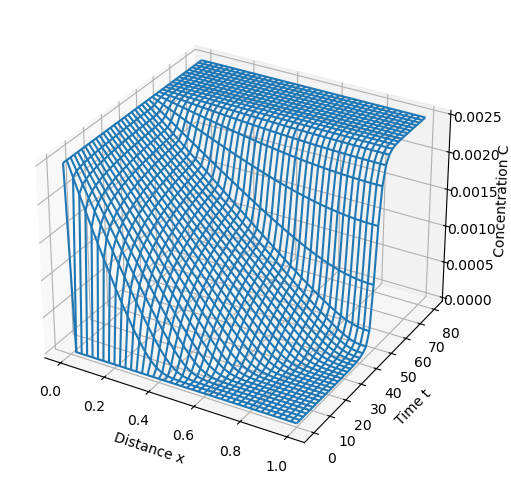
# visualization
model_plot(m)
5.4.6. Dimensional analysis#
Assuming \(L\) is determined by the experimental apparatus, choose
which results in a one parameter model
where \(\alpha = q K\) represents a dimensionless capacity of the substrate to absorb the diffusing molecule.
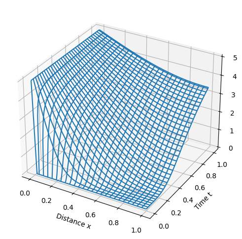
5.4.7. Dimensionless Pyomo model#
import pyomo.environ as pyo
import pyomo.dae as dae

# parameters
tf = 1.00
Cs = 5.0
alpha = 5.0

m = pyo.ConcreteModel()

m.t = dae.ContinuousSet(bounds=(0, tf))
m.x = dae.ContinuousSet(bounds=(0, 1))

m.c = pyo.Var(m.t, m.x)
m.s = pyo.Var(m.t, m.x)

m.dcdt = dae.DerivativeVar(m.c, wrt=m.t)
m.dcdx = dae.DerivativeVar(m.c, wrt=m.x)
# m.d2cdx2 = dae.DerivativeVar(m.c, wrt=(m.x, m.x))
m.d2cdx2 = dae.DerivativeVar(m.dcdx, wrt=m.x)


@m.Constraint(m.t, m.x)
def pde(m, t, x):
    if t == 0:
        return pyo.Constraint.Skip
    return m.dcdt[t, x] * (1 + alpha / (1 + m.c[t, x]) ** 2) == m.d2cdx2[t, x]


@m.Constraint(m.t)
def bc1(m, t):
    return m.c[t, 0] == Cs


@m.Constraint(m.t)
def bc2(m, t):
    return m.dcdx[t, 1] == 0


@m.Constraint(m.x)
def ic(m, x):
    if (x == 0) or (x == 1):
        return pyo.Constraint.Skip
    return m.c[0, x] == 0.0


# transform and solve
pyo.TransformationFactory("dae.finite_difference").apply_to(m, wrt=m.x, nfe=50)
pyo.TransformationFactory("dae.finite_difference").apply_to(m, wrt=m.t, nfe=100)

# Remove final degree of freedom
m.dcdx[0, 0].fix(0.0)

print("Degrees of Freedom:", degrees_of_freedom(m))
Degrees of Freedom: 0
dt = DiagnosticsToolbox(m)
dt.report_structural_issues()
dt.display_underconstrained_set()
dt.display_overconstrained_set()
====================================================================================
Model Statistics

        Activated Blocks: 1 (Deactivated: 0)
        Free Variables in Activated Constraints: 20551 (External: 0)
            Free Variables with only lower bounds: 0
            Free Variables with only upper bounds: 0
            Free Variables with upper and lower bounds: 0
        Fixed Variables in Activated Constraints: 1 (External: 0)
        Activated Equality Constraints: 20551 (Deactivated: 0)
        Activated Inequality Constraints: 0 (Deactivated: 0)
        Activated Objectives: 0 (Deactivated: 0)

------------------------------------------------------------------------------------
1 WARNINGS

    WARNING: Found 5100 potential evaluation errors.

------------------------------------------------------------------------------------
2 Cautions

    Caution: 1 variable fixed to 0
    Caution: 5203 unused variables (0 fixed)

------------------------------------------------------------------------------------
Suggested next steps:

    display_potential_evaluation_errors()

====================================================================================
====================================================================================
Dulmage-Mendelsohn Under-Constrained Set

====================================================================================
====================================================================================
Dulmage-Mendelsohn Over-Constrained Set

====================================================================================
pyo.SolverFactory("ipopt").solve(m, tee=True).write()

model_plot(m)
Ipopt 3.13.2:

******************************************************************************
This program contains Ipopt, a library for large-scale nonlinear optimization.
 Ipopt is released as open source code under the Eclipse Public License (EPL).
         For more information visit http://projects.coin-or.org/Ipopt

This version of Ipopt was compiled from source code available at
    https://github.com/IDAES/Ipopt as part of the Institute for the Design of
    Advanced Energy Systems Process Systems Engineering Framework (IDAES PSE
    Framework) Copyright (c) 2018-2019. See https://github.com/IDAES/idaes-pse.

This version of Ipopt was compiled using HSL, a collection of Fortran codes
    for large-scale scientific computation.  All technical papers, sales and
    publicity material resulting from use of the HSL codes within IPOPT must
    contain the following acknowledgement:
        HSL, a collection of Fortran codes for large-scale scientific
        computation. See http://www.hsl.rl.ac.uk.
******************************************************************************

This is Ipopt version 3.13.2, running with linear solver ma27.

Number of nonzeros in equality constraint Jacobian...:    61150
Number of nonzeros in inequality constraint Jacobian.:        0
Number of nonzeros in Lagrangian Hessian.............:    10200

Total number of variables............................:    20551
                     variables with only lower bounds:        0
                variables with lower and upper bounds:        0
                     variables with only upper bounds:        0
Total number of equality constraints.................:    20551
Total number of inequality constraints...............:        0
        inequality constraints with only lower bounds:        0
   inequality constraints with lower and upper bounds:        0
        inequality constraints with only upper bounds:        0

iter    objective    inf_pr   inf_du lg(mu)  ||d||  lg(rg) alpha_du alpha_pr  ls
   0  0.0000000e+00 5.00e+00 0.00e+00  -1.0 0.00e+00    -  0.00e+00 0.00e+00   0
   1  0.0000000e+00 4.99e+00 0.00e+00  -1.0 1.25e+04    -  1.00e+00 1.95e-03h 10
   2  0.0000000e+00 4.98e+00 0.00e+00  -1.0 1.25e+04    -  1.00e+00 1.95e-03h 10
   3  0.0000000e+00 4.97e+00 0.00e+00  -1.0 1.25e+04    -  1.00e+00 1.95e-03h 10
   4  0.0000000e+00 4.96e+00 0.00e+00  -1.0 1.24e+04    -  1.00e+00 1.95e-03h 10
   5  0.0000000e+00 4.95e+00 0.00e+00  -1.0 1.24e+04    -  1.00e+00 1.95e-03h 10
   6  0.0000000e+00 4.94e+00 0.00e+00  -1.0 1.24e+04    -  1.00e+00 1.95e-03h 10
   7  0.0000000e+00 4.93e+00 0.00e+00  -1.0 1.24e+04    -  1.00e+00 1.95e-03h 10
   8  0.0000000e+00 4.92e+00 0.00e+00  -1.0 1.23e+04    -  1.00e+00 1.95e-03h 10
   9  0.0000000e+00 4.91e+00 0.00e+00  -1.0 1.23e+04    -  1.00e+00 1.95e-03h 10
iter    objective    inf_pr   inf_du lg(mu)  ||d||  lg(rg) alpha_du alpha_pr  ls
  10  0.0000000e+00 4.90e+00 0.00e+00  -1.0 1.23e+04    -  1.00e+00 1.95e-03h 10
  11  0.0000000e+00 1.24e+03 0.00e+00  -1.0 1.23e+04    -  1.00e+00 1.00e+00w  1
  12  0.0000000e+00 2.74e+01 0.00e+00  -1.0 1.19e+03    -  1.00e+00 1.00e+00w  1
  13  0.0000000e+00 5.64e-01 0.00e+00  -1.0 1.85e+01    -  1.00e+00 1.00e+00h  1
  14  0.0000000e+00 1.54e-03 0.00e+00  -1.7 3.02e-01    -  1.00e+00 1.00e+00h  1
  15  0.0000000e+00 2.23e-08 0.00e+00  -3.8 7.66e-04    -  1.00e+00 1.00e+00h  1
  16  0.0000000e+00 3.84e-13 0.00e+00  -9.0 8.37e-09    -  1.00e+00 1.00e+00h  1

Number of Iterations....: 16

                                   (scaled)                 (unscaled)
Objective...............:   0.0000000000000000e+00    0.0000000000000000e+00
Dual infeasibility......:   0.0000000000000000e+00    0.0000000000000000e+00
Constraint violation....:   3.8369307731045410e-13    3.8369307731045410e-13
Complementarity.........:   0.0000000000000000e+00    0.0000000000000000e+00
Overall NLP error.......:   3.8369307731045410e-13    3.8369307731045410e-13


Number of objective function evaluations             = 118
Number of objective gradient evaluations             = 17
Number of equality constraint evaluations            = 120
Number of inequality constraint evaluations          = 0
Number of equality constraint Jacobian evaluations   = 17
Number of inequality constraint Jacobian evaluations = 0
Number of Lagrangian Hessian evaluations             = 16
Total CPU secs in IPOPT (w/o function evaluations)   =      1.755
Total CPU secs in NLP function evaluations           =      0.029

EXIT: Optimal Solution Found.
# ==========================================================
# = Solver Results                                         =
# ==========================================================
# ----------------------------------------------------------
#   Problem Information
# ----------------------------------------------------------
Problem:
- Lower bound: -inf
  Upper bound: inf
  Number of objectives: 1
  Number of constraints: 20551
  Number of variables: 20551
  Sense: unknown
# ----------------------------------------------------------
#   Solver Information
# ----------------------------------------------------------
Solver:
- Status: ok
  Message: Ipopt 3.13.2\x3a Optimal Solution Found
  Termination condition: optimal
  Id: 0
  Error rc: 0
  Time: 1.8977868556976318
# ----------------------------------------------------------
#   Solution Information
# ----------------------------------------------------------
Solution:
- number of solutions: 0
  number of solutions displayed: 0