None

This notebook contains material from CBE60499; content is available on Github.

< 3.0 Unconstrained Nonlinear Optimization: Theory and Algorithms | Contents | Tag Index | 3.2 Mathematics Primer >

3.1 Linear Algebra Review and SciPy Basics

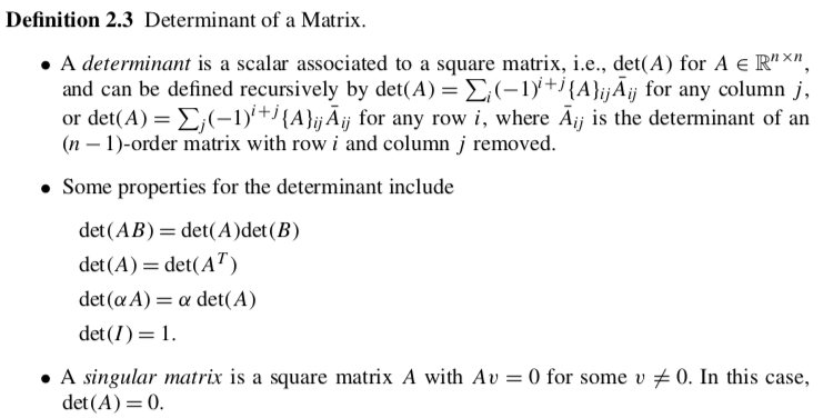
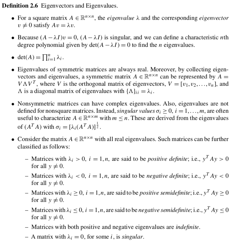
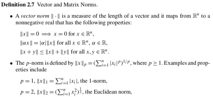
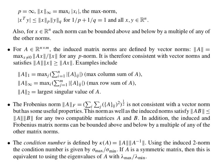
Screenshots from Section 2.2 Vectors and Matrices in Biegler (2010)

Recommended Links

• NumPy Documentation - Main Page
• SciPy Documentation - Main Page
• SciPy Linear Algebra - Tutorial
• SciPy Linear Algebra - API
• SciPy Lecture Notes (Especially 1.1 - 1.6 for everyone and 2.1 - 2.2 for advanced users)

Tip: We will mostly use SciPy for linear algebra. (It has more sophisticated capabilities than NumPy.) We will use NumPy if/when SciPy does not offer a specific command.

# Load required Python libraries.
import matplotlib.pyplot as plt
import numpy as np
from scipy import linalg

3.1.1 Notation (for textbook)

• Scalar constants and variables - Greek letters
• Vectors - Lower case Roman letters
• Matrices - Upper case Roman letters

The notation for lectures will (hopefully) be obvious from context. I sometimes use Greek letters for constants and Roman letters for variables... unless the Greek letters have engineering or scientific meaning.

Matrix Operations

# Generate random matrices
n = 2
m = 3

Ao = np.random.rand(n,m)
Bo = np.random.rand(m,n)

print("Ao = ")
print(Ao)
print("\nBo = ")
print(Bo)


# What is the dimension of A*B? Try to answer this without the computer.

# Calculate A*B using Python
print("\nAo*Bo =")
print(Ao.dot(Bo))

Ao = 
[[0.90471685 0.17317304 0.40300532]
 [0.63393766 0.90146479 0.61500922]]

Bo = 
[[0.34621818 0.9393221 ]
 [0.67416793 0.95718324]
 [0.61310823 0.40727659]]

Ao*Bo =
[[0.67706301 1.17971349]
 [1.20428661 1.7088175 ]]

Activity

• Calculate $A_o^{T}$
• Create a square matrix and check if it is symmetric
• Create a 3x3 identity matrix

# Transpose
print("transpose(Ao) = \n",Ao.transpose(),"\n")

# Create a square matrix. Is it symmetric?

# Identify matrix
print("I = \n",np.identity(3),"\n")

transpose(Ao) = 
 [[0.90471685 0.63393766]
 [0.17317304 0.90146479]
 [0.40300532 0.61500922]] 

I = 
 [[1. 0. 0.]
 [0. 1. 0.]
 [0. 0. 1.]] 

3.1.2 Determinant

# Generate random matrices
nd = 2

Ad = np.random.rand(nd,nd)
Bd = np.random.rand(nd,nd)

Cd = np.array([(1, 0, 0),(-2, 0, 0),(0, 1, 1)])

print("Ad = ")
print(Ad)
print("\nBd = ")
print(Bd)
print("\nCd = ")
print(Cd)

Ad = 
[[0.35144304 0.40331999]
 [0.98819481 0.83989719]]

Bd = 
[[0.24359748 0.02035267]
 [0.32634249 0.99856976]]

Cd = 
[[ 1  0  0]
 [-2  0  0]
 [ 0  1  1]]

Activity

• Verify the properties listed under Some properties for the determinant include
• If $A_d$, $B_d$ or $C_d$ singular?

# Property 1
print("det(A*B) = ",linalg.det(Ad.dot(Bd)))

print("det(A)*det(B) = ",linalg.det(Ad)*linalg.det(Bd))

det(A*B) =  -0.024461085784763897
det(A)*det(B) =  -0.02446108578476388

# Property 2

# Property 3

# Property 4

Another Example (for at home)

Below is an example from Linear Algebra and Its Applications by David C. Lay, 3rd edition that shows how to calculate a determinant by hand.

3.1.3 Rank

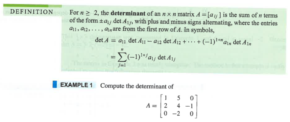
Activity

• Predict the rank of $A_o^T$, $B_o^T$, $A_d$, $B_d$, $C_d$
• Calculate np.linalg.matrix_rank(). Where you correct?

print("rank(A_o) = ",np.linalg.matrix_rank(Ao),"\n")

# Fill in remainder here.

rank(A_o) =  2 

3.1.4 Inverse

Activity

1. Calculate the inverse of $A_o$ and verity that $A_o^{-1} A_o = I$
2. Verify that det($A^{-1}$) = 1/det($A$)
3. Is $Q$ an orthogonal matrix?

# Task 1

# Task 2

# Task 3
# Is this an orthogonal matrix? Yes, no, or need more information?
theta = 0.2
Q = np.array([(np.cos(theta), -np.sin(theta)),(np.sin(theta),np.cos(theta))])

print("Q = ")
print(Q)

Q = 
[[ 0.98006658 -0.19866933]
 [ 0.19866933  0.98006658]]

3.1.5 Solving Linear Systems

Consider the linear system $A_l x = b_l$

Al = np.array([(4,3),(6,3)])
bl = np.array([1,0])
print("Al = \n",Al)
print("\nbl = \n",bl)

Al = 
 [[4 3]
 [6 3]]

bl = 
 [1 0]

3.1.5.1 Explicit Inverse

Calculate $x$ by explicitly using $A_l^{-1}$. Hint: Use linalg.inv().

Ainv = linalg.inv(Al)
print("Ainv = \n",Ainv,"\n")

# Now calculate and print x

Ainv = 
 [[-0.5         0.5       ]
 [ 1.         -0.66666667]] 

3.1.5.2 LU Decomposition

Perform LU decomposition on $A_l$. What structures do the $P$, $L$, and $U$ matrices have?

# Create test linear systems
A = np.random.rand(4,4)
print("A = \n",A,"\n")

b = np.random.rand(4,1)
print("b = \n",b,"\n")

A = 
 [[0.68331246 0.29422836 0.22419151 0.41620186]
 [0.05988483 0.58705665 0.07246852 0.45441375]
 [0.6024749  0.36997327 0.13872522 0.45388322]
 [0.34311843 0.47101812 0.51826738 0.25525007]] 

b = 
 [[0.00949348]
 [0.82027783]
 [0.90273651]
 [0.37915841]] 

# Perform LU decomposition
(P, L, U) = linalg.lu(A)

# Permutation matrix
print("P = \n",P)

# Lower diagonal matrix
print("L = \n",L)

# Upper diagonal matrix
print("U = \n",U)

# Verify result
print("P*L*U = \n",P.dot(L.dot(U)),"\n")

P = 
 [[1. 0. 0. 0.]
 [0. 1. 0. 0.]
 [0. 0. 0. 1.]
 [0. 0. 1. 0.]]
L = 
 [[ 1.          0.          0.          0.        ]
 [ 0.08763901  1.          0.          0.        ]
 [ 0.50213986  0.5759686   1.          0.        ]
 [ 0.88169751  0.19696885 -0.18479522  1.        ]]
U = 
 [[ 0.68331246  0.29422836  0.22419151  0.41620186]
 [ 0.          0.56127076  0.05282059  0.41793823]
 [ 0.          0.          0.37526888 -0.19446077]
 [ 0.          0.          0.         -0.03133716]]
P*L*U = 
 [[0.68331246 0.29422836 0.22419151 0.41620186]
 [0.05988483 0.58705665 0.07246852 0.45441375]
 [0.6024749  0.36997327 0.13872522 0.45388322]
 [0.34311843 0.47101812 0.51826738 0.25525007]] 

3.1.5.2.1 Is P orthogonal?

print("inv(P) = \n",linalg.inv(P),"\n")

print("transpose(P) = \n",P.T,"\n")

print("P.T*P = \n",np.matmul(P.T,P),"\n")

inv(P) = 
 [[ 1. -0. -0.  0.]
 [ 0.  1. -0.  0.]
 [ 0.  0. -0.  1.]
 [ 0.  0.  1.  0.]] 

transpose(P) = 
 [[1. 0. 0. 0.]
 [0. 1. 0. 0.]
 [0. 0. 0. 1.]
 [0. 0. 1. 0.]] 

P.T*P = 
 [[1. 0. 0. 0.]
 [0. 1. 0. 0.]
 [0. 0. 1. 0.]
 [0. 0. 0. 1.]] 

Yes! We see that $P^T = P^{-1}$ and $P^T \cdot P = I$.

3.1.5.2.2 MATLAB

Defines LU decomposition as follows:

$$ P \cdot A = L \cdot U$$

Consider $$A \cdot x=b$$

Using MATLAB LU definition

$$P\cdot A = L\cdot U$$$$P^T \cdot P \cdot A = P^T \cdot L \cdot U$$$$A = P^T \cdot L \cdot U$$

Substitute into linear system:

$$P^T \cdot L \cdot U \cdot x = b$$$$ L \cdot U \cdot x = P \cdot b$$

Let $y = U \cdot x$ and substitute.

Step 1. Solve $L \cdot y = P \cdot b$ for $y$

Step 2. Solve $U \cdot x = y$ for $x$

Pb = P.dot(b)
print("P*b = ",Pb,"\n")

yLU = linalg.solve(L,Pb)
print("yLU = ",yLU,"\n")

xLU = linalg.solve(U,yLU)
print("xLU = ",xLU,"\n")

P*b =  [[0.00949348]
 [0.82027783]
 [0.37915841]
 [0.90273651]] 

yLU =  [[ 0.00949348]
 [ 0.81944583]
 [-0.09758371]
 [ 0.71492782]] 

xLU =  [[  9.4407442 ]
 [ 19.58501477]
 [-12.08206663]
 [-22.81406129]] 

3.1.5.2.3 SciPy

Defines LU decomposition as:

$$ A = P \cdot L \cdot U $$

Consider $$A \cdot x=b$$

SciPy LU definition

$$A = P \cdot L\cdot U$$

Substitute into linear system:

$$P \cdot L \cdot U \cdot x = b$$$$P^T \cdot P \cdot L \cdot U \cdot x = P^T \cdot b$$$$L \cdot U \cdot x = P^T \cdot b$$

Let $y = U \cdot x$ and substitute.

Step 1. Solve $L \cdot y = P^T \cdot b$ for $y$

Step 2. Solve $U \cdot x = y$ for $x$

## LU decomposition algorithm.
Pb = (P.T).dot(b)
print("P.T*b = ",Pb,"\n")

yLU = linalg.solve(L,Pb)
print("yLU = ",yLU,"\n")

xLU = linalg.solve(U,yLU)
print("xLU = ",xLU,"\n")

P.T*b =  [[0.00949348]
 [0.82027783]
 [0.37915841]
 [0.90273651]] 

yLU =  [[ 0.00949348]
 [ 0.81944583]
 [-0.09758371]
 [ 0.71492782]] 

xLU =  [[  9.4407442 ]
 [ 19.58501477]
 [-12.08206663]
 [-22.81406129]] 

What is the difference? A transpose.

3.1.5.2.4 Verify our answer with linalg.solve

Solve the linear system using linalg.solve

x = linalg.solve(Al,bl)
print("x = \n",x)

x = 
 [-0.5  1. ]

3.1.6 Invertable Matrix Theorem

Screenshots from Linear Algebra and Its Applications by David C. Lay, 3rd edition

3.1.7 Eigenvectors and Eigenvalues

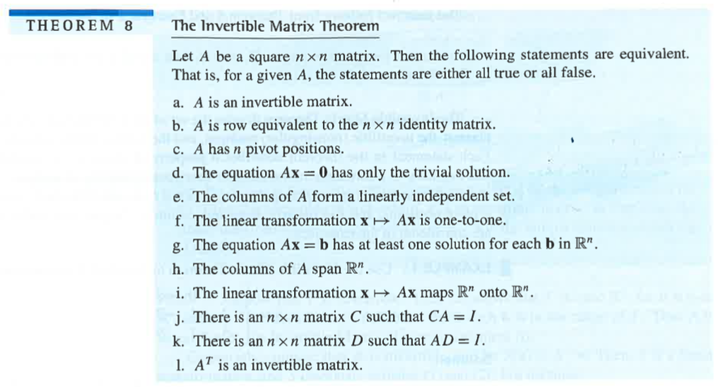
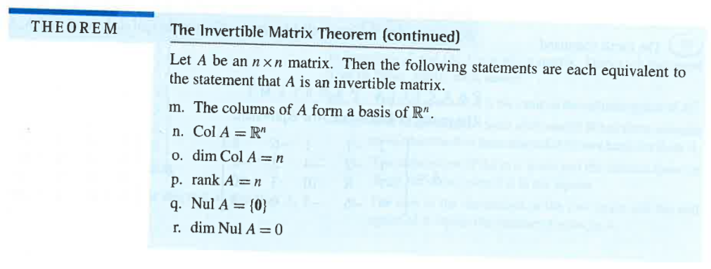
Ae = np.array([(0, -4, -6), (-1, 0, -3), (1, 2, 5)])
print("Ae = \n",Ae)

Ae = 
 [[ 0 -4 -6]
 [-1  0 -3]
 [ 1  2  5]]

Activity

• Do you expect this matrix to have negative eigenvalues? Choose: Yes / No / Cannot tell from inspection.
• Calculate the eigenvalues.
• Based on your calculations above, is this matrix i) positive definite, ii) positive semi definite, iii) negative definite, iv) negative semi definite, v) indefinite, or vi) cannot say without additional calculations? Write a sentence to justify your answer.
• Calculate the determinate using only the eigenvalues.

# Expect negative eigenavalues?
# Yes / No / Cannot tell from inspect?
# Write a sentence to justify your answer.

### Calculate eigenvalues

# Matrix Al
print("Matrix = \n",Al,"\n")
l, v = linalg.eig(Al)
print("Eigenvalues = ",l,"\n")
print("Eigenvectors = \n",v,"\n")

Matrix = 
 [[4 3]
 [6 3]] 

Eigenvalues =  [ 7.77200187+0.j -0.77200187+0.j] 

Eigenvectors = 
 [[ 0.62246561 -0.53222953]
 [ 0.78264715  0.8466001 ]] 

3.1.8 Singular Value Decomposition

Notes will be given in class.

Activity

• Calculate singular value decomposition of $A_l$ and $C_d$
• What is the rank of each matrix?

# Matrix Al
print("Matrix = \n",Al,"\n")
U,s,Vh = linalg.svd(Al)
print("U = \n",U,"\n")
print("S = \n",s,"\n")
print("Vh = \n",Vh,"\n")

## Rank (from inspecting singular values)?

Matrix = 
 [[4 3]
 [6 3]] 

U = 
 [[-0.59581566 -0.80312122]
 [-0.80312122  0.59581566]] 

S = 
 [8.33557912 0.71980602] 

Vh = 
 [[-0.86400595 -0.50348159]
 [ 0.50348159 -0.86400595]] 

3.1.9 Vector and Matrix Norms

x = np.random.rand(3,1)
print("x = \n",x)

y = np.random.rand(3,1)
print("y = \n",y)

x = 
 [[0.02808233]
 [0.20488865]
 [0.77425602]]
y = 
 [[0.73113614]
 [0.20737529]
 [0.97754014]]

Activity

• Verify the vector norm properties hold for the p-2 norm using $x$ and $y$. Hint: linalg.norm()
• Calculate $||A_l||_1$, $||A_l||_{\infty}$ and $||A_l||_2$ using both the rules given above and SciPy

3.1.10 Condition Number

Activity

• Estimate the condition number of $A_l$ by inspecting the SVD results.
• Calculate the condition number of $A_l$ using np.linalg.cond()

< 3.0 Unconstrained Nonlinear Optimization: Theory and Algorithms | Contents | Tag Index | 3.2 Mathematics Primer >