Vehicle Routing - Optimization for Decision Science

Prepared by: William Bartel (wbartel@nd.edu, 2024) and Andrew Brooks (abrooks7@nd.edu, 2024)

Learning Objectives¶

Practice with Combinatorial (MILP) Problems
Practice with Stochastic Programming
Learning how to make graph visualizations

Imports¶

# This code cell installs packages on Colab

import sys

if "google.colab" in sys.modules:
    !wget "https://raw.githubusercontent.com/ndcbe/optimization/main/notebooks/helper.py"
    import helper

    helper.easy_install()
else:
    sys.path.insert(0, "../")
    import helper
helper.set_plotting_style()

## Import Libraries
import pyomo.environ as pyo
import pandas as pd

Problem Statement and Solution¶

We are given four locations (A,B,C,D) and a depot (0). A vehicle starts at the depot and can travel on a road between any two locations. We are given the cost (we can imagine this as distance or fuel) to travel between any two locations by the given matrix, where the row is the starting location and the column is the ending location. We note this is generally a symmetric matrix, but in a general context may not be symmetric in the case of road closures or traffic.

The goal is to find a route for the vehicle starting and ending at the depot where each location is visited exactly once. This is known as the Traveling Salesman Problem, and the solution is an NP-hard problem. We seek to create a Pyomo implementation of the problem.

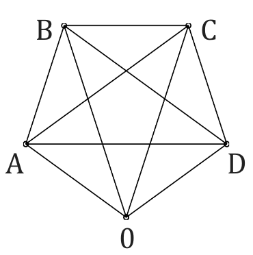
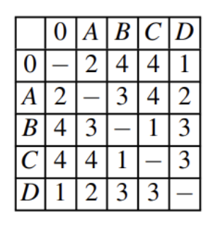
Image Source: Birge, John R., and François Louveaux. Introduction to Stochastic Programming. 2nd ed., Springer New York, 2011, p. 41, Birge & Louveaux (2011).

Initial Implementation¶

First, we will attempt an initial solution. Let us define the problem:

Sets: $L=\{0,A,B,C,D\}$

Parameters: $c_{i,j} =$ distance from $i$ to $j$ for $i,j\in L$ as determined by matrix

Variables: $x_{i,j} = 1$ if vehicle travels from $i$ to $j$ with $i,j\in L$ . Otherwise, $x_{i,j}=0$ .

Objective:

\text{min}~\sum_{i\in L}\sum_{j \in L}c_{i,j} x_{i,j}

(1)

Constraints:

\sum_{j\in L}x_{i,j}-\sum_{j\in L}x_{j,i}=0, \forall i\in L

(2)

\sum_{j\in L}x_{i,j}=1, \forall i\in L

(3)

x_{i,i}=0, \forall i\in L

(4)

Variables: 25

Constraints: 15

DOF: $25-15=10$

The set contains the locations, and the parameters store the cost of traveling between two locations as given by the matrix. If the vehicle travels between locations $i$ and $j$ , then $x_{i,j}=1$ and the total cost increases by $c_{i,j}$ . So, the objective is to minimize the sum $c_{i,j} x_{i,j}$ over all such $i$ and $j$ .

The first constraint ensures the number of entries into a location equals the number of exits out of that location. The second constraint imposes that each location is exited exactly once. The final constraint gives that a vehicle cannot travel from a location to the same location.

We import the package networkx so that we can create a function to graph our solutions as directed graphs. This gives a picture where each arrow shows the route the vehicle travels. Then, we program the problem using Pyomo and solve.

import networkx as nx
import matplotlib.pyplot as plt


# Function for visualizing data
def createGraph(model, e):
    # Create a directed graph
    G = nx.DiGraph()

    # Add some nodes and edges
    G.add_nodes_from(L)

    edges = []

    if e == []:
        for i in L:
            for j in L:
                if pyo.value(model.x[i, j]) > 0.5:
                    edges.append((i, j))
    else:
        edges = e

    G.add_edges_from(edges)

    pos = nx.circular_layout(G)

    nx.draw_networkx_edges(
        G, pos, edgelist=G.edges(), arrowstyle="->", arrowsize=20, width=2
    )
    labels = {node: "0" if node == "Depot" else node for node in G.nodes()}

    # Draw the graph
    nx.draw(G, pos, with_labels=True, labels=labels)
    plt.show()

# create model and define cost of each path
model = pyo.ConcreteModel()
L = ["Depot", "A", "B", "C", "D"]
c = {
    ("Depot", "Depot"): 0,
    ("Depot", "A"): 2,
    ("Depot", "B"): 4,
    ("Depot", "C"): 4,
    ("Depot", "D"): 1,
    ("A", "Depot"): 2,
    ("A", "A"): 0,
    ("A", "B"): 3,
    ("A", "C"): 4,
    ("A", "D"): 2,
    ("B", "Depot"): 4,
    ("B", "A"): 3,
    ("B", "B"): 0,
    ("B", "C"): 1,
    ("B", "D"): 3,
    ("C", "Depot"): 4,
    ("C", "A"): 4,
    ("C", "B"): 1,
    ("C", "C"): 0,
    ("C", "D"): 3,
    ("D", "Depot"): 1,
    ("D", "A"): 2,
    ("D", "B"): 3,
    ("D", "C"): 3,
    ("D", "D"): 0,
}

# Decision variable x of which paths are chosen is binary
model.x = pyo.Var(L, L, domain=pyo.Binary)


# Set objective to the total cost of the path
@model.Objective()
def obj(m):
    return sum(c[i, j] * m.x[i, j] for i in L for j in L)


model.cons = pyo.ConstraintList()

for i in L:
    model.cons.add(
        expr=sum(model.x[i, j] for j in L) - sum(model.x[j, i] for j in L) == 0
    )  # Entries = Exits
    model.cons.add(expr=sum(model.x[i, j] for j in L) == 1)  # Exits = 1
    model.cons.add(
        expr=model.x[i, i] == 0
    )  # No traveling from location to same location

results = pyo.SolverFactory("appsi_highs").solve(model)
assert pyo.check_optimal_termination(results), (
    f"Solve failed: status={results.solver.status}, "
    f"termination={results.solver.termination_condition}"
)

model.pprint()

createGraph(model, [])

1 Var Declarations
    x : Size=25, Index={Depot, A, B, C, D}*{Depot, A, B, C, D}
        Key                : Lower : Value : Upper : Fixed : Stale : Domain
                ('A', 'A') :     0 :   0.0 :     1 : False : False : Binary
                ('A', 'B') :     0 :  -0.0 :     1 : False : False : Binary
                ('A', 'C') :     0 :   0.0 :     1 : False : False : Binary
                ('A', 'D') :     0 :   1.0 :     1 : False : False : Binary
            ('A', 'Depot') :     0 :  -0.0 :     1 : False : False : Binary
                ('B', 'A') :     0 :  -0.0 :     1 : False : False : Binary
                ('B', 'B') :     0 :   0.0 :     1 : False : False : Binary
                ('B', 'C') :     0 :   1.0 :     1 : False : False : Binary
                ('B', 'D') :     0 :   0.0 :     1 : False : False : Binary
            ('B', 'Depot') :     0 :   0.0 :     1 : False : False : Binary
                ('C', 'A') :     0 :   0.0 :     1 : False : False : Binary
                ('C', 'B') :     0 :   1.0 :     1 : False : False : Binary
                ('C', 'C') :     0 :   0.0 :     1 : False : False : Binary
                ('C', 'D') :     0 :   0.0 :     1 : False : False : Binary
            ('C', 'Depot') :     0 :   0.0 :     1 : False : False : Binary
                ('D', 'A') :     0 :  -0.0 :     1 : False : False : Binary
                ('D', 'B') :     0 :   0.0 :     1 : False : False : Binary
                ('D', 'C') :     0 :   0.0 :     1 : False : False : Binary
                ('D', 'D') :     0 :   0.0 :     1 : False : False : Binary
            ('D', 'Depot') :     0 :   1.0 :     1 : False : False : Binary
            ('Depot', 'A') :     0 :   1.0 :     1 : False : False : Binary
            ('Depot', 'B') :     0 :   0.0 :     1 : False : False : Binary
            ('Depot', 'C') :     0 :   0.0 :     1 : False : False : Binary
            ('Depot', 'D') :     0 :   0.0 :     1 : False : False : Binary
        ('Depot', 'Depot') :     0 :   0.0 :     1 : False : False : Binary

1 Objective Declarations
    obj : Size=1, Index=None, Active=True
        Key  : Active : Sense    : Expression
        None :   True : minimize : 0*x[Depot,Depot] + 2*x[Depot,A] + 4*x[Depot,B] + 4*x[Depot,C] + x[Depot,D] + 2*x[A,Depot] + 0*x[A,A] + 3*x[A,B] + 4*x[A,C] + 2*x[A,D] + 4*x[B,Depot] + 3*x[B,A] + 0*x[B,B] + x[B,C] + 3*x[B,D] + 4*x[C,Depot] + 4*x[C,A] + x[C,B] + 0*x[C,C] + 3*x[C,D] + x[D,Depot] + 2*x[D,A] + 3*x[D,B] + 3*x[D,C] + 0*x[D,D]

1 Constraint Declarations
    cons : Size=15, Index={1, 2, 3, 4, 5, 6, 7, 8, 9, 10, 11, 12, 13, 14, 15}, Active=True
        Key : Lower : Body                                                                                                                                      : Upper : Active
          1 :   0.0 : x[Depot,Depot] + x[Depot,A] + x[Depot,B] + x[Depot,C] + x[Depot,D] - (x[Depot,Depot] + x[A,Depot] + x[B,Depot] + x[C,Depot] + x[D,Depot]) :   0.0 :   True
          2 :   1.0 :                                                                        x[Depot,Depot] + x[Depot,A] + x[Depot,B] + x[Depot,C] + x[Depot,D] :   1.0 :   True
          3 :   0.0 :                                                                                                                            x[Depot,Depot] :   0.0 :   True
          4 :   0.0 :                                         x[A,Depot] + x[A,A] + x[A,B] + x[A,C] + x[A,D] - (x[Depot,A] + x[A,A] + x[B,A] + x[C,A] + x[D,A]) :   0.0 :   True
          5 :   1.0 :                                                                                            x[A,Depot] + x[A,A] + x[A,B] + x[A,C] + x[A,D] :   1.0 :   True
          6 :   0.0 :                                                                                                                                    x[A,A] :   0.0 :   True
          7 :   0.0 :                                         x[B,Depot] + x[B,A] + x[B,B] + x[B,C] + x[B,D] - (x[Depot,B] + x[A,B] + x[B,B] + x[C,B] + x[D,B]) :   0.0 :   True
          8 :   1.0 :                                                                                            x[B,Depot] + x[B,A] + x[B,B] + x[B,C] + x[B,D] :   1.0 :   True
          9 :   0.0 :                                                                                                                                    x[B,B] :   0.0 :   True
         10 :   0.0 :                                         x[C,Depot] + x[C,A] + x[C,B] + x[C,C] + x[C,D] - (x[Depot,C] + x[A,C] + x[B,C] + x[C,C] + x[D,C]) :   0.0 :   True
         11 :   1.0 :                                                                                            x[C,Depot] + x[C,A] + x[C,B] + x[C,C] + x[C,D] :   1.0 :   True
         12 :   0.0 :                                                                                                                                    x[C,C] :   0.0 :   True
         13 :   0.0 :                                         x[D,Depot] + x[D,A] + x[D,B] + x[D,C] + x[D,D] - (x[Depot,D] + x[A,D] + x[B,D] + x[C,D] + x[D,D]) :   0.0 :   True
         14 :   1.0 :                                                                                            x[D,Depot] + x[D,A] + x[D,B] + x[D,C] + x[D,D] :   1.0 :   True
         15 :   0.0 :                                                                                                                                    x[D,D] :   0.0 :   True

3 Declarations: x obj cons

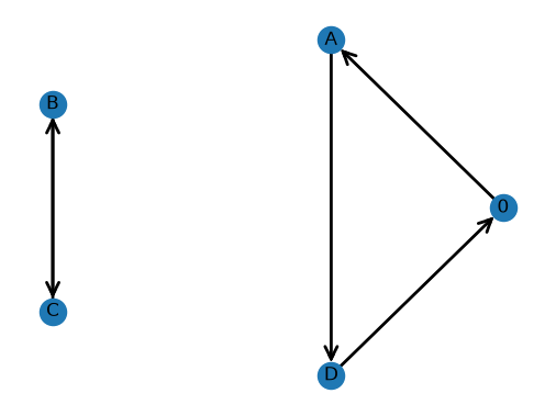
We notice that our initial implementation failed. Our constraints did not require for a route to be connected, so the solution generated two separate loops. We need to add another set of constraints to address connectedness.

MTZ Constraints and Full Solution¶

To address connectedness, we implement Miller-Tucker-Zemlin constraints. These are a set of constraints to ensure our solution outputs a connected graph.

First, we add a new variable $u_{i}$ for $i\in\{A,B,C,D\}$ , where $u_{i}$ is equal to the order in which we visit location $i$ . For example, if the route of the vehicle is $0\rightarrow A\rightarrow C\rightarrow D\rightarrow B\rightarrow 0$ , then $u_{A}=1, u_{C}=2, u_{D}=3, u_{B}=4$ . We omit 0 as an index for $u_i$ , since this would create confusion as to whether $u_0=0$ or $u_0=5$ with the constraints we plan to add.

First, we implement two new constraints

u_i\geq 1, \hspace{2mm}\forall i\in \{A,B,C,D\}

(5)

u_i\leq \text{len}(L)-1,\hspace{2mm} \forall i\in \{A,B,C,D\}

(6)

We use len $(L)$ in a general case, but for this specific problem, len $(L)=5$ , so we have $u_i\leq 4$ . These constraints will ensure that for the 4 locations the vehicle will visit, each integer value 1 through 4 will be associated to a $u_i$ for $i\in\{A,B,C,D\}$ . Next, we add one more constraint

u_i-u_j+(\text{len}(L)-1)x_{i,j}\leq \text{len}(L)-2, \hspace{2mm}\forall i\forall j\in \{A,B,C,D\},i\neq j

(7)

If $x_{i,j}=0$ , this statement imposes $u_i-u_j\leq\text{len}(L)-2$ which does not restrict $u_i$ or $u_j$ at all. If $x_{i,j}=1$ , then $u_i-u_j\leq-1$ , so $u_j>u_i$ . Combined with the boundary constraints on each $u_i$ , this will force $u_j=u_i+1$ if $x_{i,j}=1$ .

Now, we implement these constraints and solve the model.

Full Model:

Sets:

$L=\{0,A,B,C,D\}$

Parameters:

$c_{i,j} =$ distance from $i$ to $j$ for $i,j\in L$ as determined by matrix

Variables:

$x_{i,j} = 1$ if vehicle travels from $i$ to $j$ with $i,j\in L$ . Otherwise, $x_{i,j}=0$ .

$u_i =$ the order in which the car visits location $i$ for $i\in \{A,B,C,D\}$

Objective:

\text{min}\sum_{i\in L}\sum_{j \in L}c_{i,j}x_{i,j}

(8)

Constraints:

\sum_{j\in L}x_{i,j}-\sum_{j\in L}x_{j,i}=0, \forall i\in L

(9)

\sum_{j\in L}x_{i,j}=1, \forall i\in L

(10)

x_{i,i}=0, \forall i\in L

(11)

u_i-u_j+(\text{len}(L)-1)x_{i,j}\leq \text{len}(L)-2, \hspace{2mm}\forall i\forall j\in \{A,B,C,D\},i\neq j

(12)

u_i\geq 1, \hspace{2mm}\forall i\in \{A,B,C,D\}

(13)

u_i\leq \text{len}(L)-1,\hspace{2mm} \forall i\in \{A,B,C,D\}

(14)

Variables: $4+25=29$

Constraints: $15+12=27$

DOF: $29-27=2$

# Subtour elimination (MTZ constraints)
model.u = pyo.Var(["A", "B", "C", "D"], domain=pyo.NonNegativeReals)

# Ensure values of u are sequential
for i in L:
    for j in L:
        if i != j and i != "Depot" and j != "Depot":
            model.cons.add(
                model.u[i] - model.u[j] + (len(L) - 1) * model.x[i, j] <= len(L) - 2
            )  # Connected cities have u values differ by 1

# Set a range for u variables
for i in L:
    if i != "Depot":
        model.cons.add(model.u[i] >= 1)
        model.cons.add(model.u[i] <= len(L) - 1)

results = pyo.SolverFactory("appsi_highs").solve(model)
assert pyo.check_optimal_termination(results), (
    f"Solve failed: status={results.solver.status}, "
    f"termination={results.solver.termination_condition}"
)

model.pprint()

print()

createGraph(model, [])

2 Var Declarations
    u : Size=4, Index={A, B, C, D}
        Key : Lower : Value : Upper : Fixed : Stale : Domain
          A :     0 :   4.0 :  None : False : False : NonNegativeReals
          B :     0 :   3.0 :  None : False : False : NonNegativeReals
          C :     0 :   2.0 :  None : False : False : NonNegativeReals
          D :     0 :   1.0 :  None : False : False : NonNegativeReals
    x : Size=25, Index={Depot, A, B, C, D}*{Depot, A, B, C, D}
        Key                : Lower : Value : Upper : Fixed : Stale : Domain
                ('A', 'A') :     0 :   0.0 :     1 : False : False : Binary
                ('A', 'B') :     0 :   0.0 :     1 : False : False : Binary
                ('A', 'C') :     0 :   0.0 :     1 : False : False : Binary
                ('A', 'D') :     0 :   0.0 :     1 : False : False : Binary
            ('A', 'Depot') :     0 :   1.0 :     1 : False : False : Binary
                ('B', 'A') :     0 :   1.0 :     1 : False : False : Binary
                ('B', 'B') :     0 :   0.0 :     1 : False : False : Binary
                ('B', 'C') :     0 :   0.0 :     1 : False : False : Binary
                ('B', 'D') :     0 :   0.0 :     1 : False : False : Binary
            ('B', 'Depot') :     0 :   0.0 :     1 : False : False : Binary
                ('C', 'A') :     0 :   0.0 :     1 : False : False : Binary
                ('C', 'B') :     0 :   1.0 :     1 : False : False : Binary
                ('C', 'C') :     0 :   0.0 :     1 : False : False : Binary
                ('C', 'D') :     0 :   0.0 :     1 : False : False : Binary
            ('C', 'Depot') :     0 :   0.0 :     1 : False : False : Binary
                ('D', 'A') :     0 :   0.0 :     1 : False : False : Binary
                ('D', 'B') :     0 :   0.0 :     1 : False : False : Binary
                ('D', 'C') :     0 :   1.0 :     1 : False : False : Binary
                ('D', 'D') :     0 :   0.0 :     1 : False : False : Binary
            ('D', 'Depot') :     0 :   0.0 :     1 : False : False : Binary
            ('Depot', 'A') :     0 :   0.0 :     1 : False : False : Binary
            ('Depot', 'B') :     0 :   0.0 :     1 : False : False : Binary
            ('Depot', 'C') :     0 :   0.0 :     1 : False : False : Binary
            ('Depot', 'D') :     0 :   1.0 :     1 : False : False : Binary
        ('Depot', 'Depot') :     0 :   0.0 :     1 : False : False : Binary

1 Objective Declarations
    obj : Size=1, Index=None, Active=True
        Key  : Active : Sense    : Expression
        None :   True : minimize : 0*x[Depot,Depot] + 2*x[Depot,A] + 4*x[Depot,B] + 4*x[Depot,C] + x[Depot,D] + 2*x[A,Depot] + 0*x[A,A] + 3*x[A,B] + 4*x[A,C] + 2*x[A,D] + 4*x[B,Depot] + 3*x[B,A] + 0*x[B,B] + x[B,C] + 3*x[B,D] + 4*x[C,Depot] + 4*x[C,A] + x[C,B] + 0*x[C,C] + 3*x[C,D] + x[D,Depot] + 2*x[D,A] + 3*x[D,B] + 3*x[D,C] + 0*x[D,D]

1 Constraint Declarations
    cons : Size=35, Index={1, 2, 3, 4, 5, 6, 7, 8, 9, 10, 11, 12, 13, 14, 15, 16, 17, 18, 19, 20, 21, 22, 23, 24, 25, 26, 27, 28, 29, 30, 31, 32, 33, 34, 35}, Active=True
        Key : Lower : Body                                                                                                                                      : Upper : Active
          1 :   0.0 : x[Depot,Depot] + x[Depot,A] + x[Depot,B] + x[Depot,C] + x[Depot,D] - (x[Depot,Depot] + x[A,Depot] + x[B,Depot] + x[C,Depot] + x[D,Depot]) :   0.0 :   True
          2 :   1.0 :                                                                        x[Depot,Depot] + x[Depot,A] + x[Depot,B] + x[Depot,C] + x[Depot,D] :   1.0 :   True
          3 :   0.0 :                                                                                                                            x[Depot,Depot] :   0.0 :   True
          4 :   0.0 :                                         x[A,Depot] + x[A,A] + x[A,B] + x[A,C] + x[A,D] - (x[Depot,A] + x[A,A] + x[B,A] + x[C,A] + x[D,A]) :   0.0 :   True
          5 :   1.0 :                                                                                            x[A,Depot] + x[A,A] + x[A,B] + x[A,C] + x[A,D] :   1.0 :   True
          6 :   0.0 :                                                                                                                                    x[A,A] :   0.0 :   True
          7 :   0.0 :                                         x[B,Depot] + x[B,A] + x[B,B] + x[B,C] + x[B,D] - (x[Depot,B] + x[A,B] + x[B,B] + x[C,B] + x[D,B]) :   0.0 :   True
          8 :   1.0 :                                                                                            x[B,Depot] + x[B,A] + x[B,B] + x[B,C] + x[B,D] :   1.0 :   True
          9 :   0.0 :                                                                                                                                    x[B,B] :   0.0 :   True
         10 :   0.0 :                                         x[C,Depot] + x[C,A] + x[C,B] + x[C,C] + x[C,D] - (x[Depot,C] + x[A,C] + x[B,C] + x[C,C] + x[D,C]) :   0.0 :   True
         11 :   1.0 :                                                                                            x[C,Depot] + x[C,A] + x[C,B] + x[C,C] + x[C,D] :   1.0 :   True
         12 :   0.0 :                                                                                                                                    x[C,C] :   0.0 :   True
         13 :   0.0 :                                         x[D,Depot] + x[D,A] + x[D,B] + x[D,C] + x[D,D] - (x[Depot,D] + x[A,D] + x[B,D] + x[C,D] + x[D,D]) :   0.0 :   True
         14 :   1.0 :                                                                                            x[D,Depot] + x[D,A] + x[D,B] + x[D,C] + x[D,D] :   1.0 :   True
         15 :   0.0 :                                                                                                                                    x[D,D] :   0.0 :   True
         16 :  -Inf :                                                                                                                    u[A] - u[B] + 4*x[A,B] :   3.0 :   True
         17 :  -Inf :                                                                                                                    u[A] - u[C] + 4*x[A,C] :   3.0 :   True
         18 :  -Inf :                                                                                                                    u[A] - u[D] + 4*x[A,D] :   3.0 :   True
         19 :  -Inf :                                                                                                                    u[B] - u[A] + 4*x[B,A] :   3.0 :   True
         20 :  -Inf :                                                                                                                    u[B] - u[C] + 4*x[B,C] :   3.0 :   True
         21 :  -Inf :                                                                                                                    u[B] - u[D] + 4*x[B,D] :   3.0 :   True
         22 :  -Inf :                                                                                                                    u[C] - u[A] + 4*x[C,A] :   3.0 :   True
         23 :  -Inf :                                                                                                                    u[C] - u[B] + 4*x[C,B] :   3.0 :   True
         24 :  -Inf :                                                                                                                    u[C] - u[D] + 4*x[C,D] :   3.0 :   True
         25 :  -Inf :                                                                                                                    u[D] - u[A] + 4*x[D,A] :   3.0 :   True
         26 :  -Inf :                                                                                                                    u[D] - u[B] + 4*x[D,B] :   3.0 :   True
         27 :  -Inf :                                                                                                                    u[D] - u[C] + 4*x[D,C] :   3.0 :   True
         28 :   1.0 :                                                                                                                                      u[A] :  +Inf :   True
         29 :  -Inf :                                                                                                                                      u[A] :   4.0 :   True
         30 :   1.0 :                                                                                                                                      u[B] :  +Inf :   True
         31 :  -Inf :                                                                                                                                      u[B] :   4.0 :   True
         32 :   1.0 :                                                                                                                                      u[C] :  +Inf :   True
         33 :  -Inf :                                                                                                                                      u[C] :   4.0 :   True
         34 :   1.0 :                                                                                                                                      u[D] :  +Inf :   True
         35 :  -Inf :                                                                                                                                      u[D] :   4.0 :   True

4 Declarations: x obj cons u

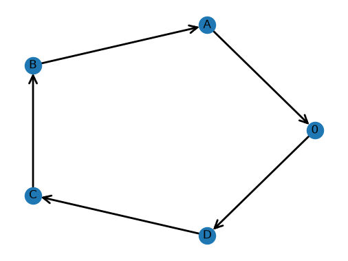
We obtain a solution that is connected and minimizes the cost of travel for the vehicle.

Integer Cuts¶

We utilize integer cuts to obtain the 7 best solutions to the problem. After we solve the model, we create two sets:

A:=\{(i,j): x_{i,j}=1\}

(15)

B:=\{(i,j): x_{i,j}=0\}

(16)

Then, after each time we solve the model, we add a new constraint to the model:

\sum_{(i,j)\in A}x_{i,j}+\sum_{(i,j)\in B}(1-x_{i,j})\leq \text{len}(L)^2-1

(17)

Since there are $\text{len}(L)^2$ combinations of choosing $i,j\in L$ , then requiring this sum to be less than or equal to $\text{len}(L)^2-1$ ensures we cannot have a duplicate solution if we resolve the model.

Repeating this process, we obtain the 7 best solutions (7 is chosen arbitrarily here, and we can do this to find the top $n$ solutions for any $n$ ).

# Declare the ConstraintList outside the loop
model.int_cuts = pyo.ConstraintList()

for k in range(0, 7):
    results = pyo.SolverFactory("appsi_highs").solve(model)
    assert pyo.check_optimal_termination(results), (
        f"Solve failed: status={results.solver.status}, "
        f"termination={results.solver.termination_condition}"
    )

    print(f"Objective: {pyo.value(model.obj)}")

    A = []
    B = []

    # Use a tolerance rather than == 1, because the solver returns floats
    for i in L:
        for j in L:
            if pyo.value(model.x[i, j]) > 0.5:
                A.append([i, j])
            else:
                B.append([i, j])

    edges = [(i, j) for i, j in A]

    createGraph(model, edges)

    # Add a new constraint to the existing ConstraintList
    model.int_cuts.add(
        expr=sum(model.x[i[0], i[1]] for i in A)
        + sum(1 - model.x[i[0], i[1]] for i in B)
        <= pow(len(L), 2) - 1
    )
    print()

Objective: 10.0

Objective: 10.0

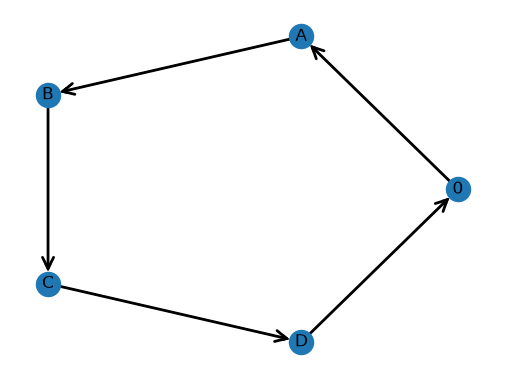
Objective: 11.0

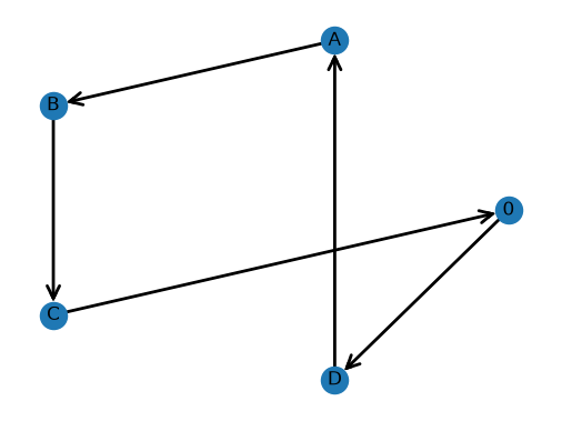
Objective: 11.0

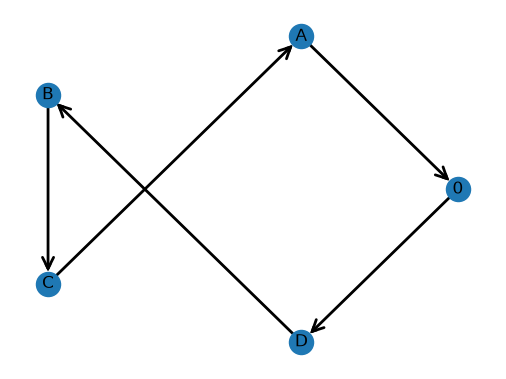
Objective: 11.0

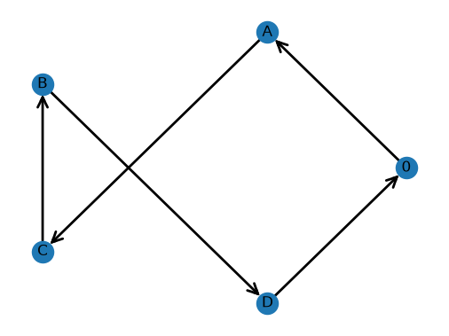
Objective: 11.0

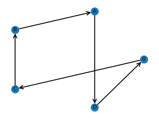
Objective: 12.0

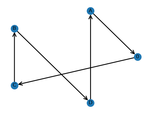
We obtain 2 solutions that have a cost of 10, and 4 solutions that have a cost of 11. The final solution we obtain has a cost of 12, and there are more routes with cost equal to 12 that would come next if we looked at the next best routes.

We notice that for any given route, we can traverse the route backwards to obtain another route that gives the same cost to travel. This is because our matrix of costs is symmetric.

Extension Problem¶

To introduce stochastic variables into the problem, we used a formulation found online. It can be found here: https://github.com/Pyomo/pyomo-model-libraries/tree/main/pysp/vehicle_routing/3-7b.

In this related problem, which is also a combinatorial problem, the challenge is to determine the routing of a fleet of cars to a number of nodes in order to maximize the revenue while travelling from five starting points and all ending at node 20. The first stage variable is deciding how many cars to start at each of the five vehicle starting points. The stochastic variable is the demand on each path, which is not known at the time of choosing the starting spot of the vehicles. The second stage variable is the actual routing decisions once the demands of each path is known. This simulates how a company may have to choose how many vehicles to buy for each warehouse location. They can only buy a certain amount of vehicles, and they want to optimize their decision based on the possible demands of the surrounding area. The demands may change day-to-day, but they can probabilistically choose the best solution.

A visual depiction of the problem is shown below. The starting points are 1-5 and the end node is 20.

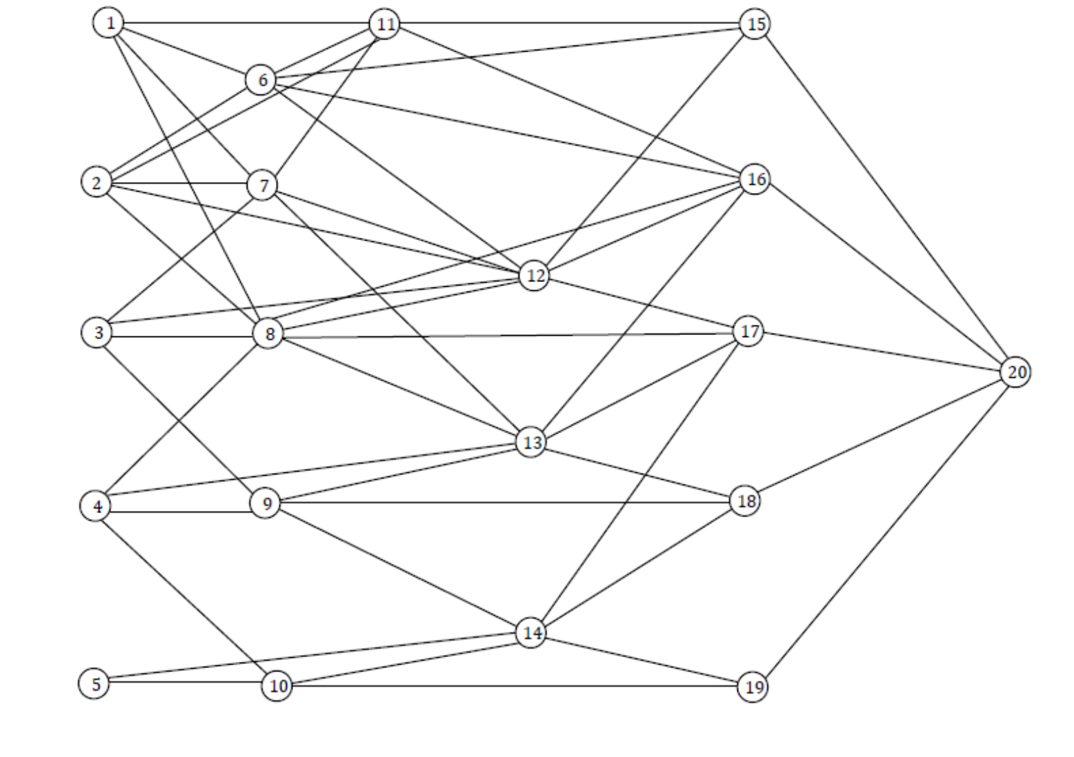
Image Source: UTPySP Examples, Pyomo Model Libraries, GitHub, p. 20, pysp/UTPySPExamples.pdf. Accessed October 2024.

Sets:

$E =$ set of edges $(i,j)$ in network

$S =$ set of source (starting) nodes

$D =$ set of demand nodes

$\Omega =$ set of scenarios

Parameters:

$c_e =$ cost on edge $(i,j)=e\in E$

$r_e =$ revenue on edge $(i,j)=e\in E$

$b =$ total number of vehicles

Random Variables:

$d_e =$ demand on edge $(i,j)=e\in E$

Decision Variables:

$x_s =$ first stage number of vehicles at source node $s$

$y_e^\omega =$ second stage routing for scenario $\omega$

$z_e^\omega =$ second stage overage for scenario $\omega$

Objective:

\text{max}\sum_{\Omega,E}\{p^\omega r_e y_e^\omega - (r_e+c_e)z_e^\omega\}

(18)

Constraints:

\sum_{s}x_{s}=b

(19)

\sum_{j\in J,(i,j)\in E}y_{(i,j)}^\omega=x_i,\hspace{5mm}\forall i\in S,\omega\in\Omega

(20)

\sum_{j\in J|(i,j)\in E}y_{(i,j)}^\omega=\sum_{i\in I|(j,i)\in E}y_{(j,i)}^\omega,\hspace{5mm}\forall j\in D,\omega\in\Omega

(21)

y_e^\omega-d_e^\omega\leq z_e^\omega,\hspace{5mm}\forall e\in E,\omega\in\Omega

(22)

0\leq\{x,y,z\}\leq b

(23)

Variables: $|S|+2|E||\Omega|$

Constraints: $1+|S||\Omega|+|D||\Omega|+|E||\Omega|$

DOF: $|S|-1+|\Omega|(|E|-|S|-|D|)$

The objective is to maximize profit. The constraints ensure (in order) that all vehicles are assigned, an enforcement of flow from the assigned vehicles at the source nodes, balance of flow at demand nodes, and excess supply at each node. All variables are nonnegative and bounded by the number of total available vehicles.

#
# Model
#
model = pyo.AbstractModel()

#
# Parameters
#
# Define sets
model.I = pyo.Set()  # node
model.J = pyo.Set()
model.S = pyo.Set()  # source node
model.D = pyo.Set()  # demand node

# Data_deterministic
model.Arc = pyo.Param(model.I, model.J)  # arc available
model.Rev = pyo.Param(model.I, model.J)  # arc revenue
model.Cost = pyo.Param(model.I, model.J)  # arc cost
model.B = pyo.Param()

# Data_stochastic
model.ArcDemand = pyo.Param(model.I, model.J)  # arc demand


# Variables
model.X = pyo.Var(model.S, bounds=(0.0, model.B), domain=pyo.NonNegativeIntegers)
model.Y = pyo.Var(
    model.I, model.J, bounds=(0.0, model.B), domain=pyo.NonNegativeIntegers
)
model.Z = pyo.Var(model.I, model.J, bounds=(0.0, None))

model.FirstStageProfit = pyo.Var()
model.SecondStageProfit = pyo.Var()


# Constraints
def vehicle_num_cap_rule(model):
    return sum(model.X[s] for s in model.S) == model.B


model.VehicleNumCapRule = pyo.Constraint(rule=vehicle_num_cap_rule)


def vehicle_assigned_cap_rule(model, s):
    return sum(model.Y[s, j] for j in model.J if model.Arc[s, j] >= 1) == model.X[s]


model.RequiredDemandRule = pyo.Constraint(model.S, rule=vehicle_assigned_cap_rule)


def flow_balance_rule(model, d):
    return (
        sum(model.Y[i, d] for i in model.I if model.Arc[i, d] >= 1)
        - sum(model.Y[d, i] for i in model.I if model.Arc[d, i] >= 1)
    ) == 0.0


model.FlowBalanceRule = pyo.Constraint(model.D, rule=flow_balance_rule)


def overage_rule(model, i, j):
    return model.Y[i, j] - model.ArcDemand[i, j] <= model.Z[i, j]


model.OverageRule = pyo.Constraint(model.I, model.J, rule=overage_rule)


def y_rule(model, i, j):
    return (0.0, model.Y[i, j], model.Arc[i, j] * 51)


model.YRule = pyo.Constraint(model.I, model.J, rule=y_rule)


# Stage-specific cost computations
def first_stage_profit_rule(model):
    return model.FirstStageProfit == 0.0


model.ComputeFirstStageProfit = pyo.Constraint(rule=first_stage_profit_rule)


def second_stage_profit_rule(model):
    return (
        model.SecondStageProfit
        - sum(
            sum(
                model.Rev[i, j] * model.Y[i, j]
                - (model.Rev[i, j] + model.Cost[i, j]) * model.Z[i, j]
                for i in model.I
            )
            for j in model.J
        )
        == 0.0
    )


model.ComputeSecondStageProfit = pyo.Constraint(rule=second_stage_profit_rule)


# Objective
def total_profit_rule(model):
    return model.FirstStageProfit + model.SecondStageProfit


model.Total_Profit_Objective = pyo.Objective(rule=total_profit_rule, sense=pyo.maximize)

# Solve and print
# with open('ReferenceModel.dat', 'r') as file:
#     data = file.read()
EV_model = model.create_instance("ReferenceModel.dat")
opt = pyo.SolverFactory("appsi_highs")
results = opt.solve(EV_model)
assert pyo.check_optimal_termination(results), (
    f"Solve failed: status={results.solver.status}, "
    f"termination={results.solver.termination_condition}"
)
EV = pyo.value(EV_model.Total_Profit_Objective)
print("EV = %.2f" % (EV))
print("Amount of vehicles at each starting point")
for i in EV_model.X:
    # X is NonNegativeIntegers, but the solver returns a float that can sit a
    # few ULPs off a whole number (e.g. 10.99999999999997). Round for display.
    print("%s = %d" % (i, round(pyo.value(EV_model.X[i]))))

EV = 17482.55
Amount of vehicles at each starting point
1 = 11
2 = 16
3 = 7
4 = 11
5 = 6

Conclusion¶

We went beyond the material from the textbook by creating our own implementation and then learning about MTZ constraints to solve the problem. To learn more about stochastic programming, we found and implemented an extension of the problem that was more complex and made use of a stochastic variable.

References¶

Birge, John R., and François Louveaux. Introduction to Stochastic Programming. 2nd ed., Springer New York, 2011, Birge & Louveaux (2011).

Pyomo Model Libraries, GitHub, https://github.com/Pyomo/pyomo-model-libraries/tree/main/pysp/vehicle_routing/3-7b. Accessed October 2024.

“Miller-Tucker-Zemlin Formulation.” AIMMS How-To, 19 Nov. 2020, how-to.aimms.com/Articles/332/332-Miller-Tucker-Zemlin-formulation.html. Accessed October 2024.

Stewart, William R., and Bruce L. Golden. ‘Stochastic Vehicle Routing: A Comprehensive Approach’. European Journal of Operational Research, vol. 14, no. 4, 1983, pp. 371–385, Stewart & Golden (1983).

References¶

Birge, J. R., & Louveaux, F. (2011). Introduction to Stochastic Programming. In Springer Series in Operations Research and Financial Engineering. Springer New York. 10.1007/978-1-4614-0237-4
Stewart, W. R., Jr., & Golden, B. L. (1983). Stochastic vehicle routing: A comprehensive approach. European Journal of Operational Research, 14(4), 371–385. 10.1016/0377-2217(83)90237-0