Parameter estimation with parmest

Created by Kanishka Ghosh, Jialu Wang, Prof. Alex Dowling, and Stephen Cini at the University of Notre Dame. Last updated December 2024.

# This code cell installs packages on Colab
import sys

if "google.colab" in sys.modules:
    !wget "https://raw.githubusercontent.com/ndcbe/optimization/main/notebooks/helper.py"
    import helper

    helper.install_idaes()
    helper.install_ipopt()
else:
    sys.path.insert(0, "../")
    import helper
helper.set_plotting_style()

import numpy as np
import matplotlib.pyplot as plt
import pandas as pd
import pyomo.environ as pyo
import pyomo.dae as dae
import pyomo
import idaes

# Define the directory to save/read the data files
data_dir = "https://raw.githubusercontent.com/ndcbe/optimization/main/notebooks/data/"

What is parameter estimation?¶

Given a function $f(x,\theta)$ where $x$ is the input or array of inputs, $\theta$ is the vector of unknown model parameters, and $y$ is the array of observed output, parameter estimation is performed to determine the values of $\theta$ to minimize the error between $f(x,\theta)$ and $y$ . Commonly, parameter estimation is set up as a least squares objective problem:

\begin{align} \begin{split} \min_{\hat{\theta}} \quad & \sum_{i}^{} (y_i - f(x_i,\hat{\theta}))^2\\ \textrm{s.t.} \quad & \mathrm{bounds \ on} \ \theta\\ & \mathrm{other \ physical \ constraints}\\ \end{split} \end{align}

(1)

where $i$ is used to index the datapoints in a dataset and $\hat{\theta}$ is the optimal set of parameter values that minimizes the prediction error.

What is `parmest`?¶

parmest is a Python package built on the Pyomo optimization modeling language to support parameter estimation using experimental data along with confidence regions and subsequent creation of scenarios for PySP. parmest supports scenario generation for multiple ‘experiments’ and can be used to characterize estimate uncertainties through, for example, confidence region generations. parmest requires the following positional arguments in order solve the optimization problem:

Experiment class with the following functions:
init - Loads data into class, and initializes model to contain no information.
create_model - Define the model in a generic form with needed variables and parameters.
finalize_model - Initialize and/or discretize the model from create_model for use with specified data.
label_model - Add required labels. parmest requires the model contains labeled unknown_parameters and model_outputs. pyomo.DoE additionally requires model_inputs and measurement_error.
get_labeled_model - Calls previous functions to generate complete model for each Experiment.
Optional keyword argument to define the verbosity of solver output. Default: False

More information about the parmest package can be found here.

Detailed explanation of the various methods in parmest can be found here.

Example: Reaction Kinetics¶

Consider two chemical reactions that convert molecule $A$ to desired product $B$ and a less valuable side-product $C$ .

A \overset{k_1}{\rightarrow} B \overset{k_2}{\rightarrow} C

(2)

Our ultimate goal is to design a large-scale continuous reactor that maximizes the production of $B$ . This general sequential reactions problem is widely applicable to CO $_2$ capture and industry more broadly (petrochemicals, pharmaceuticals, etc.).

The rate laws for these two chemical reactions are:

r_A = -k_1 C_A

(3)

r_B = k_1 C_A - k_2 C_B

(4)

r_C = k_2 C_B

(5)

Here, $C_A$ , $C_B$ , and $C_C$ are the concentrations of each species. The rate constants $k_1$ and $k_2$ depend on temperature as follows:

k_1 = A_1 \exp{\frac{-E_1}{R T}}

(6)

k_2 = A_2 \exp{\frac{-E_2}{R T}}

(7)

$A_1, A_2, E_1$ , and $E_2$ are fitted model parameters. $R$ is the ideal-gas constant and $T$ is absolute temperature.

Batch Reactor¶

The concentrations in a batch reactor evolve with time per the following differential equations:

\frac{d C_A}{dt} = r_A = -k_1 C_A

(8)

\frac{d C_B}{dt} = r_B = k_1 C_A - k_2 C_B

(9)

\frac{d C_C}{dt} = r_C = k_2 C_B

(10)

This is a linear system of differential equations. Assuming the feed is only species $A$ , i.e.,

C_A(t=0) = C_{A0} \quad C_B(t=0) = 0 \quad C_C(t=0) = 0

(11)

leads to the following analytic solution:

C_A(t) = C_{A,0} \exp(-k_1 t)

(12)

C_B(t) = \frac{k_1}{k_2 - k_1} C_{A,0} \left[\exp(-k_1 t) - \exp(-k_2 t) \right]

(13)

C_C(t) = C_{A,0} - \frac{k_2}{k_2 - k_1} C_{A,0} \exp(-k_1 t) + \frac{k_1}{k_2 - k_1} \exp(-k_2 t) C_{A,0} = C_{A,0} - C_{A}(t) - C_{B}(t)

(14)

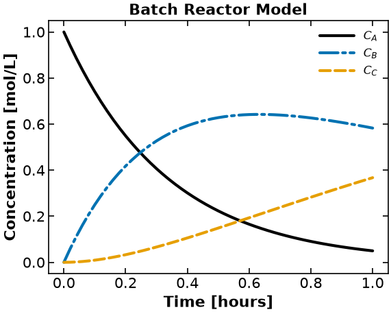
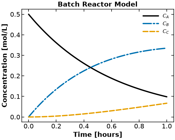
The following Python code simulates and plots this model.

def kinetics(A, E, T):
    """Computes kinetics from Arrhenius equation

    Arguments:
        A: pre-exponential factor, [1 / hr]
        E: activation energy, [kJ / mol]
        T: temperature, [K]

    Returns:
        k: reaction rate coefficient, [1 / hr]

    """
    R = 8.31446261815324  # J / K / mole

    return A * np.exp(-E * 1000 / (R * T))


def concentrations(t, k, CA0):
    """
    Returns concentrations at time t

    Arguments:
        t: time, [hr]
        k: reaction rate coefficient, [1 / hr]
        CA0: initial concentration of A, [mol / L]

    Returns:
        CA, CB, CC: concentrations of A, B, and C at time t, [mol / L]
    """
    CA = CA0 * np.exp(-k[0] * t)
    CB = k[0] * CA0 / (k[1] - k[0]) * (np.exp(-k[0] * t) - np.exp(-k[1] * t))
    CC = CA0 - CA - CB

    return CA, CB, CC

CA0 = 1  # Moles/L
k = [3, 0.7]  # 1/hr

t = np.linspace(0, 1, 51)
CA, CB, CC = concentrations(t, k, CA0)
plt.plot(t, CA, label="$C_{A}$", linestyle="-", color="blue")
plt.plot(t, CB, label="$C_{B}$", linestyle="-.", color="green")
plt.plot(t, CC, label="$C_{C}$", linestyle="--", color="red")
plt.xlabel("Time [hours]")
plt.ylabel("Concentration [mol/L]")
plt.title("Batch Reactor Model")
plt.legend()
plt.show()
plt.close()

Experimental Data¶

See the notebook Supplementary material: data for parmest tutorial for details on how these experimental data were generated (via simulation).

Experimental data consists of the concentration of species A, B, and C in $\mathrm{mol/L}$ with respect to time $t$ in $\mathrm{hours}$ inside the batch reactor. The experimental data is stored in csv files where the first column records the time $t$ in the reactor. Next, the temperature $T$ in $\mathrm{K}$ at which the reaction was simulated is recorded followed by the initial concentration of species A, $C_{A,0}$ , in $\mathrm{mol/L}$ . Finally, the time-varying species concentrations ( $C_A$ ), ( $C_B$ ), and ( $C_C$ ) are recorded in $\mathrm{mol/L}$ . Following is how the pandas dataframe of a single experiment looks like:

# define function to plot
def plot_exp(k, CA0, data, text):
    """
    Plot concentration profiles
    Arguments:
        k: kinetic parameters
        CA0: initial concentration
        data: Pandas data frame
        text: plot title

    """
    # evaluate models
    t = np.linspace(0, 1, 51)
    CA, CB, CC = concentrations(t, k, CA0)

    # plot model-generated and 'experimental' data
    # symbols for 'experimental' data
    # solid and dashed lines for model-generated data
    plt.plot(t, CA, label="$C_{A}$", linestyle="-", color="blue")
    plt.plot(data.time, data.CA, marker="o", linestyle="", color="blue", label=str())
    plt.plot(t, CB, label="$C_{B}$", linestyle="-.", color="green")
    plt.plot(data.time, data.CB, marker="s", linestyle="", color="green", label=str())
    plt.plot(t, CC, label="$C_{C}$", linestyle="--", color="red")
    plt.plot(data.time, data.CC, marker="^", linestyle="", color="red", label=str())
    plt.xlabel("Time [hours]")
    plt.ylabel("Concentration [mol/L]")
    plt.title(text)
    plt.legend()
    plt.show()
    plt.close()

Pyomo model¶

In the following cell, we define a function to define and return the Pyomo model for the kinetic model to be used for parameter estimation.

import pyomo.contrib.parmest.parmest as parmest
from pyomo.contrib.parmest.experiment import Experiment


def reaction_kinetics_model(data):

    # define Pyomo model
    m = pyo.ConcreteModel()
    m.T = data["T"][0]  # K
    m.CA0 = data["CA0"][0]  # mol/L
    m.R = 8.31446261815324  # J / K / mol

    # # define 'experimental' data timesteps as Pyomo set
    m.t = pyo.Set(initialize=data["time"].tolist())

    # Kinetic parameters to be fitted defined as Pyomo variables
    # Initialized by 'true' values
    m.A1 = pyo.Var(initialize=200, bounds=(100, 300))  # 1/hr
    m.A2 = pyo.Var(initialize=400, bounds=(300, 500))  # 1/hr
    m.E1 = pyo.Var(initialize=10, bounds=(1, 20))  # kJ/mol
    m.E2 = pyo.Var(initialize=15, bounds=(1, 30))  # kJ/mol

    # Concentration variables indexed by time
    m.CA = pyo.Var(m.t, initialize=m.CA0)  # mol/L
    m.CB = pyo.Var(m.t, initialize=0)  # mol/L
    m.CC = pyo.Var(m.t, initialize=0)  # mol/L

    # kinetic rate constants from Arrhenius equation
    m.k1 = pyo.Expression(rule=m.A1 * pyo.exp(-m.E1 * 1000 / (m.R * m.T)))  # 1/hr
    m.k2 = pyo.Expression(rule=m.A2 * pyo.exp(-m.E2 * 1000 / (m.R * m.T)))  # 1/hr

    # Constraints to change concentrations based on kinetics
    def conc_A(m, i):
        if i == 0:
            return pyo.Constraint.Skip
        else:
            return m.CA[i] == m.CA0 * pyo.exp(-m.k1 * i)

    m.CA_rate = pyo.Constraint(m.t, rule=conc_A)

    def conc_B(m, i):
        if i == 0:
            return pyo.Constraint.Skip
        else:
            return m.CB[i] == m.k1 * m.CA0 / (m.k2 - m.k1) * (
                pyo.exp(-m.k1 * i) - pyo.exp(-m.k2 * i)
            )

    m.CB_rate = pyo.Constraint(m.t, rule=conc_B)

    def conc_C(m, i):
        if i == 0:
            return pyo.Constraint.Skip
        else:
            return m.CC[i] == m.CA0 - m.CA[i] - m.CB[i]

    m.CC_rate = pyo.Constraint(m.t, rule=conc_C)

    return m

class ReactionKineticsExperiment(Experiment):

    def __init__(self, data):
        self.data = data
        self.model = None

    def create_model(self):
        self.model = m = reaction_kinetics_model(self.data)
        return m

    def finalize_model(self):
        m = self.model

        # Initial Conditions

        m.CA[0].fix(m.CA0)
        m.CB[0].fix(0.0)
        m.CC[0].fix(0.0)

        return m

    def label_model(self):
        m = self.model

        m.experiment_outputs = pyo.Suffix(direction=pyo.Suffix.LOCAL)
        m.experiment_outputs.update(
            (m.CA[t], self.data["CA"][ind]) for ind, t in enumerate(self.data["time"])
        )
        m.experiment_outputs.update(
            (m.CB[t], self.data["CB"][ind]) for ind, t in enumerate(self.data["time"])
        )
        m.experiment_outputs.update(
            (m.CC[t], self.data["CC"][ind]) for ind, t in enumerate(self.data["time"])
        )

        m.unknown_parameters = pyo.Suffix(direction=pyo.Suffix.LOCAL)
        m.unknown_parameters.update(
            (k, pyo.ComponentUID(k)) for k in [m.A1, m.A2, m.E1, m.E2]
        )

        # Standard deviation of the measurement noise. Pyomo 6.10 requires this
        # suffix to compute the covariance matrix (see `cov_est` below). The value
        # is `stdev_m_error` from the Parmest-generate-data notebook, which is the
        # noise that was added when these data files were generated.
        m.measurement_error = pyo.Suffix(direction=pyo.Suffix.LOCAL)
        m.measurement_error.update((k, 0.1) for k in m.experiment_outputs)
        return m

    def get_labeled_model(self):
        m = self.create_model()
        m = self.finalize_model()
        m = self.label_model()
        # m.pprint()

        return m

# Test model
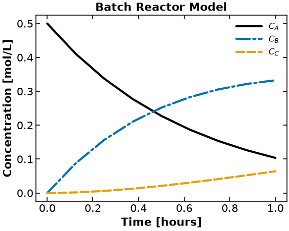
data = pd.read_csv(data_dir + "parmest_20210609_data_exp1.csv", index_col=0)
print(data)

m = reaction_kinetics_model(data)

m.CA[0].fix(m.CA0)
m.CB[0].fix(0.0)
m.CC[0].fix(0.0)

# solve model

solver = pyo.SolverFactory("ipopt")

# solve model
results = solver.solve(m, tee=True)
assert pyo.check_optimal_termination(results), (
    f"Solve failed: status={results.solver.status}, "
    f"termination={results.solver.termination_condition}"
)
# m.pprint()

# plot results
CA = [pyo.value(m.CA[i]) for i in m.t]
CB = [pyo.value(m.CB[i]) for i in m.t]
CC = [pyo.value(m.CC[i]) for i in m.t]
plt.plot(m.t, CA, label="$C_{A}$", linestyle="-", color="blue")
plt.plot(m.t, CB, label="$C_{B}$", linestyle="-.", color="green")
plt.plot(m.t, CC, label="$C_{C}$", linestyle="--", color="red")
plt.xlabel("Time [hours]")
plt.ylabel("Concentration [mol/L]")
plt.title("Batch Reactor Model")
plt.legend()

    time    T  CA0        CA        CB        CC
0  0.000  250  0.5  0.676405  0.041060  0.031307
1  0.125  250  0.5  0.447945  0.104749  0.000000
2  0.250  250  0.5  0.430686  0.306222  0.000000
3  0.375  250  0.5  0.495617  0.291236  0.078701
4  0.500  250  0.5  0.408284  0.268605  0.108478
5  0.625  250  0.5  0.083008  0.331605  0.000000
6  0.750  250  0.5  0.242464  0.342886  0.270002
7  0.875  250  0.5  0.105167  0.474409  0.000000
8  1.000  250  0.5  0.087828  0.314504  0.071406

Ipopt 3.13.2: 

******************************************************************************
This program contains Ipopt, a library for large-scale nonlinear optimization.
 Ipopt is released as open source code under the Eclipse Public License (EPL).
         For more information visit http://projects.coin-or.org/Ipopt

This version of Ipopt was compiled from source code available at
    https://github.com/IDAES/Ipopt as part of the Institute for the Design of
    Advanced Energy Systems Process Systems Engineering Framework (IDAES PSE
    Framework) Copyright (c) 2018-2019. See https://github.com/IDAES/idaes-pse.

This version of Ipopt was compiled using HSL, a collection of Fortran codes
    for large-scale scientific computation.  All technical papers, sales and
    publicity material resulting from use of the HSL codes within IPOPT must
    contain the following acknowledgement:
        HSL, a collection of Fortran codes for large-scale scientific
        computation. See http://www.hsl.rl.ac.uk.
******************************************************************************

This is Ipopt version 3.13.2, running with linear solver ma27.

Number of nonzeros in equality constraint Jacobian...:       88
Number of nonzeros in inequality constraint Jacobian.:        0
Number of nonzeros in Lagrangian Hessian.............:       10

Total number of variables............................:       28
                     variables with only lower bounds:        0
                variables with lower and upper bounds:        4
                     variables with only upper bounds:        0
Total number of equality constraints.................:       24
Total number of inequality constraints...............:        0
        inequality constraints with only lower bounds:        0
   inequality constraints with lower and upper bounds:        0
        inequality constraints with only upper bounds:        0

iter    objective    inf_pr   inf_du lg(mu)  ||d||  lg(rg) alpha_du alpha_pr  ls
   0  0.0000000e+00 4.02e-01 0.00e+00  -1.0 0.00e+00    -  0.00e+00 0.00e+00   0
   1  0.0000000e+00 5.34e-07 0.00e+00  -1.0 4.01e-01    -  9.91e-01 1.00e+00h  1
   2  0.0000000e+00 6.14e-05 0.00e+00  -1.7 5.36e-02    -  1.00e+00 1.00e+00h  1
   3  0.0000000e+00 2.72e-07 0.00e+00  -3.8 3.41e-03    -  1.00e+00 1.00e+00h  1
   4  0.0000000e+00 7.12e-07 0.00e+00  -5.7 5.52e-03    -  1.00e+00 1.00e+00h  1
   5  0.0000000e+00 8.50e-09 0.00e+00  -8.6 6.04e-04    -  1.00e+00 1.00e+00h  1

Number of Iterations....: 5

                                   (scaled)                 (unscaled)
Objective...............:   0.0000000000000000e+00    0.0000000000000000e+00
Dual infeasibility......:   0.0000000000000000e+00    0.0000000000000000e+00
Constraint violation....:   8.4954715484641952e-09    8.4954715484641952e-09
Complementarity.........:   2.6198259016630073e-09    2.6198259016630073e-09
Overall NLP error.......:   8.4954715484641952e-09    8.4954715484641952e-09


Number of objective function evaluations             = 6
Number of objective gradient evaluations             = 6
Number of equality constraint evaluations            = 6
Number of inequality constraint evaluations          = 0
Number of equality constraint Jacobian evaluations   = 6
Number of inequality constraint Jacobian evaluations = 0
Number of Lagrangian Hessian evaluations             = 5
Total CPU secs in IPOPT (w/o function evaluations)   =      0.001
Total CPU secs in NLP function evaluations           =      0.000

EXIT: Optimal Solution Found.

Parameter estimation with a single dataset¶

Here, we will estimate parameters $A_1$ , $A_2$ , $E_1$ , and $E_2$ using data generated for a batch ‘experiment’ at 250 K with an inlet concentration of 0.5 mol/L of A.

The parameter estimation problem is solved with the least squares optimization scheme $$

\begin{align} \begin{split} \min_{\hat{\theta}} \quad & \sum_{i}^{} (y_i - f(x_i,\hat{\theta}))^2\\ \textrm{s.t.} \quad & \mathrm{bounds \ on} \ \theta\\ & \mathrm{other \ physical \ constraints}\\ \end{split} \end{align}

(15)

$ $where$ i $is used to index the datapoints in a dataset and$ \hat{\theta}$ is the optimal set of parameter values that minimizes the prediction error.

# # read-in data from csv file
data = pd.read_csv(data_dir + "parmest_20210609_data_exp1.csv", index_col=0)

# # run parmest

exp_list = []
df = data

exp_list.append(ReactionKineticsExperiment(df))

pest = parmest.Estimator(exp_list, obj_function="SSE", tee=True)

obj, theta = pest.theta_est()


print("===  Parameter values  ===")
print("A1 = {:0.3f} 1/hr".format(theta["A1"]))
print("A2 = {:0.3f} 1/hr".format(theta["A2"]))
print("E1 = {:0.3f} kJ/mol".format(theta["E1"]))
print("E2 = {:0.3f} kJ/mol".format(theta["E2"]))

Ipopt 3.13.2: 

******************************************************************************
This program contains Ipopt, a library for large-scale nonlinear optimization.
 Ipopt is released as open source code under the Eclipse Public License (EPL).
         For more information visit http://projects.coin-or.org/Ipopt

This version of Ipopt was compiled from source code available at
    https://github.com/IDAES/Ipopt as part of the Institute for the Design of
    Advanced Energy Systems Process Systems Engineering Framework (IDAES PSE
    Framework) Copyright (c) 2018-2019. See https://github.com/IDAES/idaes-pse.

This version of Ipopt was compiled using HSL, a collection of Fortran codes
    for large-scale scientific computation.  All technical papers, sales and
    publicity material resulting from use of the HSL codes within IPOPT must
    contain the following acknowledgement:
        HSL, a collection of Fortran codes for large-scale scientific
        computation. See http://www.hsl.rl.ac.uk.
******************************************************************************

This is Ipopt version 3.13.2, running with linear solver ma27.

Number of nonzeros in equality constraint Jacobian...:       96
Number of nonzeros in inequality constraint Jacobian.:        0
Number of nonzeros in Lagrangian Hessian.............:       34

Total number of variables............................:       32
                     variables with only lower bounds:        0
                variables with lower and upper bounds:        4
                     variables with only upper bounds:        0
Total number of equality constraints.................:       28
Total number of inequality constraints...............:        0
        inequality constraints with only lower bounds:        0
   inequality constraints with lower and upper bounds:        0
        inequality constraints with only upper bounds:        0

iter    objective    inf_pr   inf_du lg(mu)  ||d||  lg(rg) alpha_du alpha_pr  ls
   0  1.5248996e+00 4.02e-01 2.98e-01  -1.0 0.00e+00    -  0.00e+00 0.00e+00   0
   1  2.6912302e-01 1.60e-05 1.40e-03  -1.0 4.00e-01    -  9.91e-01 1.00e+00f  1
   2  2.6835364e-01 6.39e-04 2.62e-04  -1.7 3.05e-01    -  1.00e+00 1.00e+00h  1
   3  2.6830265e-01 1.36e-04 5.00e-05  -3.8 1.61e-01    -  9.98e-01 1.00e+00h  1
   4  2.6830221e-01 2.67e-06 7.96e-07  -5.7 2.31e-02    -  1.00e+00 1.00e+00h  1
   5  2.6830221e-01 4.56e-10 1.09e-10  -8.6 6.80e-04    -  1.00e+00 1.00e+00h  1

Number of Iterations....: 5

                                   (scaled)                 (unscaled)
Objective...............:   2.6830221390502623e-01    2.6830221390502623e-01
Dual infeasibility......:   1.0924545719690344e-10    1.0924545719690344e-10
Constraint violation....:   4.5593256947640270e-10    4.5593256947640270e-10
Complementarity.........:   2.5599493217886738e-09    2.5599493217886738e-09
Overall NLP error.......:   2.5599493217886738e-09    2.5599493217886738e-09


Number of objective function evaluations             = 6
Number of objective gradient evaluations             = 6
Number of equality constraint evaluations            = 6
Number of inequality constraint evaluations          = 0
Number of equality constraint Jacobian evaluations   = 6
Number of inequality constraint Jacobian evaluations = 0
Number of Lagrangian Hessian evaluations             = 5
Total CPU secs in IPOPT (w/o function evaluations)   =      0.000
Total CPU secs in NLP function evaluations           =      0.000

EXIT: Optimal Solution Found.

===  Parameter values  ===
A1 = 199.995 1/hr
A2 = 399.938 1/hr
E1 = 10.093 kJ/mol
E2 = 15.507 kJ/mol

Parameter estimation with multiple datasets¶

Here, we will estimate parameters $A_1$ , $A_2$ , $E_1$ , and $E_2$ using data generated for a batch ‘experiment’ at 250 K with an inlet concentration of 0.5 mol/L of A.

The parameter estimation problem is now defined to solve optimization problem where the objective function is the mean of the least square error between observed and calculated data for multiple experiments.

\begin{align} \begin{split} \min_{\hat{\theta}} \quad & \frac{1}{N}\sum_{j}^{}\sum_{i}^{} (y_{j,i} - f(x_{j,i},\hat{\theta}))^2\\ \textrm{s.t.} \quad & \mathrm{bounds \ on} \ \theta\\ & \mathrm{other \ physical \ constraints}\\ \end{split} \end{align}

(16)

where $i$ is used to index the datapoints in a dataset, $j$ is an index on the dataset such that $j \in [1,N]$ and $N$ is the number of experiments conducted.

Generate Experiment list¶

In the following cell, we define a function to generate a list of Experiments using the Experiment class. For this, we read-in the list of file names generated earlier.

# Make empty experiment list
exp_list = []

# Set generic file name to fill with data 1-16
file_name_generic = data_dir + "parmest_20210609_data_exp{}.csv"

for i in range(
    16
):  # making a list of different experiments, each exp has corresponding data
    df = pd.read_csv(file_name_generic.format(i + 1), index_col=0)
    # print(df.head())
    exp_list.append(ReactionKineticsExperiment(df))

Parameter estimation with parmest¶

In the following cell, we perform parameter estimation using parmest to solve the least squares problem defined in the Pyomo model.

In Google Colab, an error appears: ‘_PyDrive2ImportHook’ object has no attribute ‘find_spec’. This is being fixed by a recent patch to Pyomo: Pyomo/pyomo#3444. Results generated using local run of software.

# run parmest

pest = parmest.Estimator(exp_list, obj_function="SSE")

obj, theta = pest.theta_est()

# print(theta)


print("===  Parameter values  ===")
print("A1 = {:0.3f} 1/hr".format(theta["A1"]))
print("A2 = {:0.3f} 1/hr".format(theta["A2"]))
print("E1 = {:0.3f} kJ/mol".format(theta["E1"]))
print("E2 = {:0.3f} kJ/mol".format(theta["E2"]))

===  Parameter values  ===
A1 = 204.414 1/hr
A2 = 390.586 1/hr
E1 = 10.046 kJ/mol
E2 = 15.021 kJ/mol

Plotting fitted model simulation with ‘experimental’ data¶

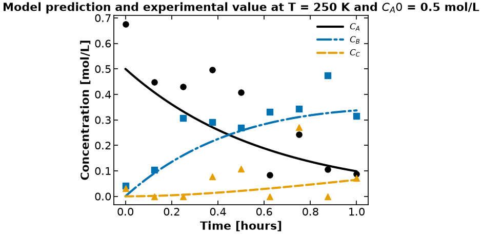
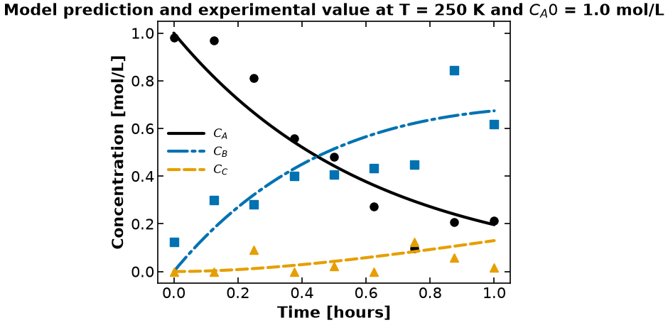
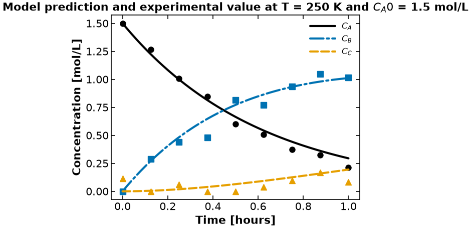
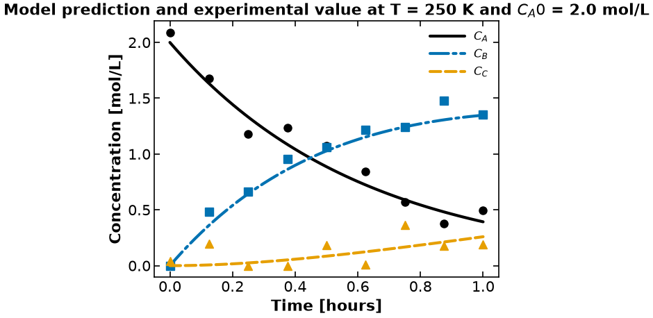
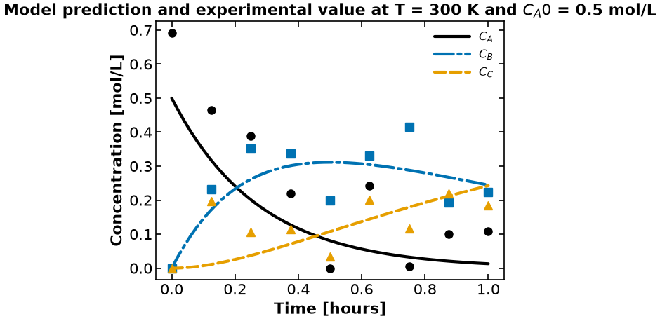
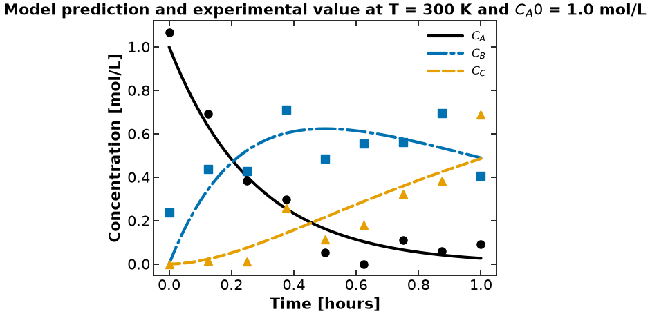
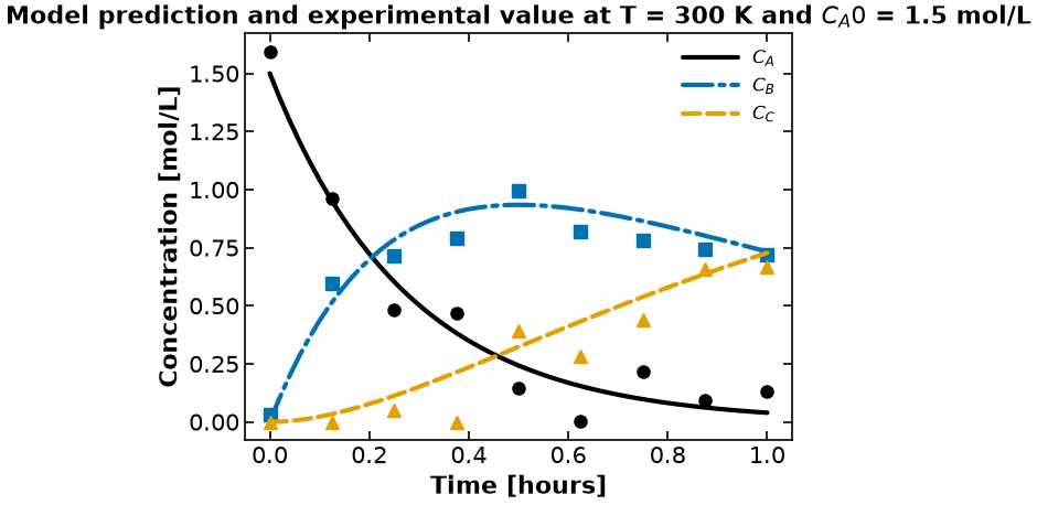
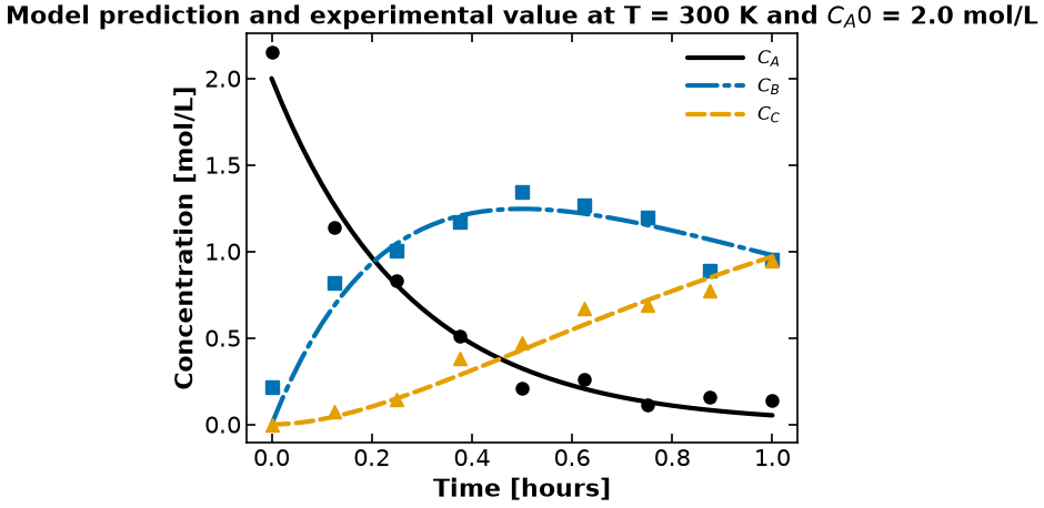
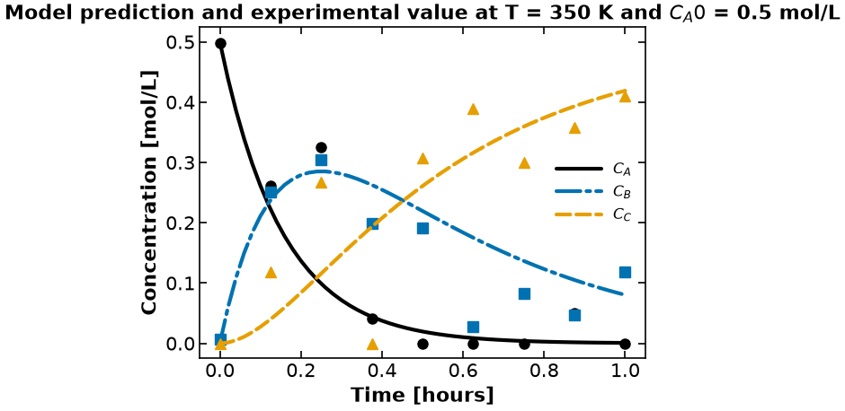
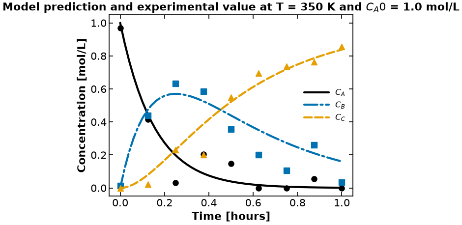
Next, we plot the ‘experimental’ data along with the profiles generated using the fitted kinetic model. The symbols represent the ‘experimental’ data and the solid and dashed lines are the profiles generated using the fitted model.

# list of temperatures
T_vals = [250, 300, 350, 400]  # K

# list of initial concentrations of A
CA0_vals = [0.5, 1.0, 1.5, 2.0]  # mol/L

# Parameter values from parameter estimation using parmest
A1 = theta["A1"]
E1 = theta["E1"]
A2 = theta["A2"]
E2 = theta["E2"]


A_est1 = [A1, A2]
A_est = np.asarray(A_est1)

E_est1 = [E1, E2]
E_est = np.asarray(E_est1)

ctr = 0
for T in T_vals:
    for CA0 in CA0_vals:
        # generate concentration profiles using estimated parameter values
        k = kinetics(A_est, E_est, T)
        # plot model-generated and 'experimental' data
        # symbols for 'experimental' data
        # solid and dashed lines for model-generated data
        df = pd.read_csv(file_name_generic.format(ctr + 1), index_col=0)
        plot_exp(
            k,
            CA0,
            df,
            "Model prediction and experimental value at T = {} K and $C_{}$ = {} mol/L".format(
                T, "A0", CA0
            ),
        )
        ctr += 1

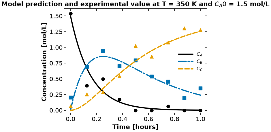
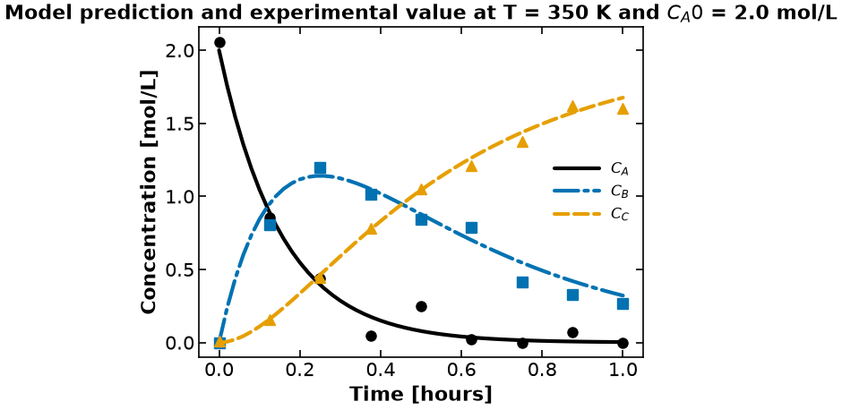
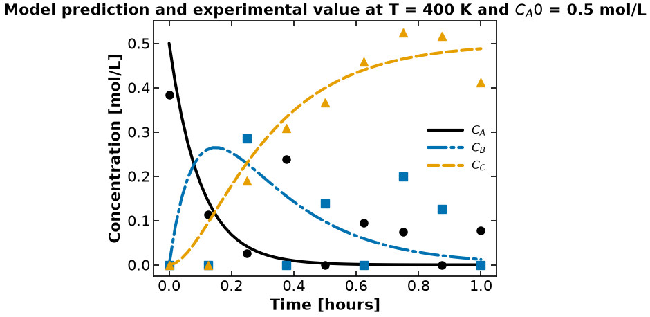
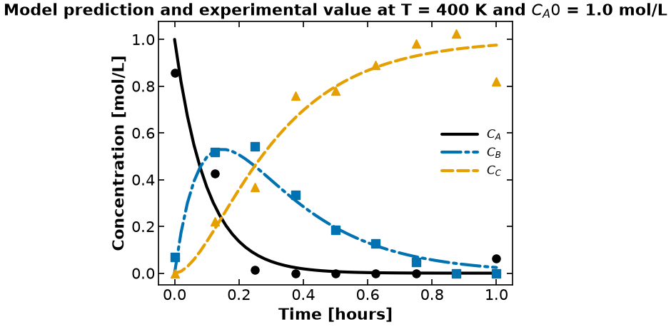
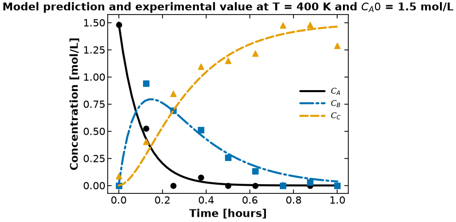
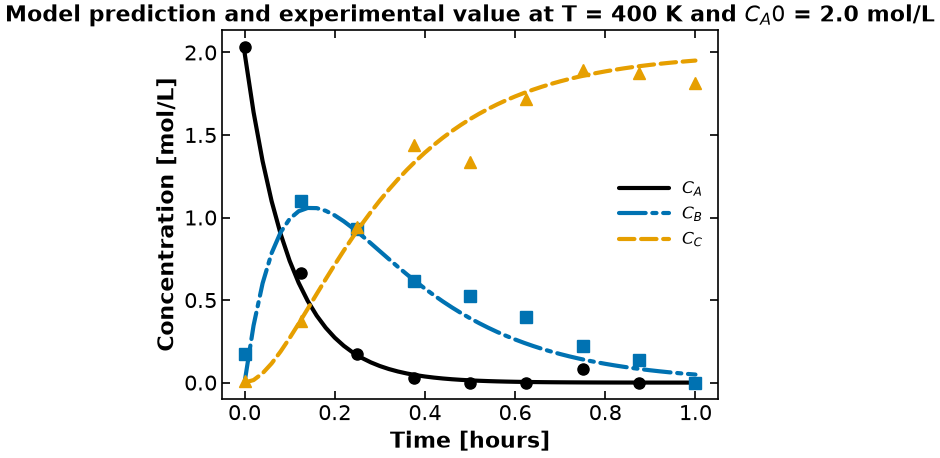
Using `parmest` with `pyomo.dae`¶

In contrast to the approach above, we will now try to solve the model without the analytic solution for the concentrations using Pyomo.DAE. To recap, the concentrations in a batch reactor evolve with time per the following differential equations:

\frac{d C_A}{dt} = r_A = -k_1 C_A

(17)

\frac{d C_B}{dt} = r_B = k_1 C_A - k_2 C_B

(18)

\frac{d C_C}{dt} = r_C = k_2 C_B

(19)

This is a linear system of differential equations. Assuming the feed is only species $A$ , i.e.,

C_A(t=0) = C_{A0} \quad C_B(t=0) = 0 \quad C_C(t=0) = 0

(20)

In the following cell, we define a function to define and return the Pyomo DAE model (dynamic mode) for the kinetic model to be used for parameter estimation. In this model, the rate equations are presented in terms of linear differential equations.

Note

A note on units. This pyomo.dae model records its units in comments (# 1/hr, # mol/L, # kJ/mol) rather than with Pyomo’s units= argument, unlike the dynamic optimization notebooks in Units in Pyomo.dae Models. That is a deliberate scope decision, not an oversight: the model is consumed by parmest, which builds the sum-of-squares objective and clones the model per experiment, and m.T is assigned as a plain Python attribute rather than a Pyomo Param. Annotating it properly means annotating the experiment data columns too.

It is worth seeing what the comments are hiding, though. The Arrhenius expression is

m.k1 = pyo.Expression(rule=m.A1 * pyo.exp(-m.E1 * 1000 / (m.R * m.T)))

That bare 1000 is a hand-rolled unit conversion: E1 is in kJ/mol and R is in J/(K·mol), so the activation energy must be multiplied by 1000 to reach joules. Nothing in the code says so. Get the factor wrong -- or drop it when you refactor -- and the model still runs, still converges, and returns confidently wrong kinetic parameters.

This is precisely the class of error assert_units_consistent exists to catch. If E1 carried units.kJ / units.mol and R carried units.J / units.K / units.mol, Pyomo would do the conversion itself and the 1000 would disappear.

The exponent’s argument must also come out dimensionless, which is a free check on the whole expression:

\frac{[\mathrm{kJ}/\mathrm{mol}] \cdot 1000} {[\mathrm{J}/(\mathrm{K}\cdot\mathrm{mol})] \cdot [\mathrm{K}]} = \frac{\mathrm{J}/\mathrm{mol}}{\mathrm{J}/\mathrm{mol}} = 1 .

(21)

And note the same ContinuousSet limitation as everywhere else: m.t is initialized from data["time"] in hours, and there is nowhere to record that. See Pyomo issue #1790.

import pyomo.contrib.parmest.parmest as parmest
from pyomo.contrib.parmest.experiment import Experiment


def reaction_kinetics_model_dae(data):

    # define Pyomo model
    m = pyo.ConcreteModel()
    m.T = data["T"][0]  # K
    m.CA0 = data["CA0"][0]  # mol/L
    m.R = 8.31446261815324  # J / K / mol

    # # define 'experimental' data timesteps as Pyomo set
    m.t = dae.ContinuousSet(initialize=data["time"].tolist(), bounds=(0, 1))

    # Kinetic parameters to be fitted defined as Pyomo variables
    # Initialized by 'true' values
    m.A1 = pyo.Var(initialize=200, bounds=(100, 300))  # 1/hr
    m.A2 = pyo.Var(initialize=400, bounds=(300, 500))  # 1/hr
    m.E1 = pyo.Var(initialize=10, bounds=(1, 20))  # kJ/mol
    m.E2 = pyo.Var(initialize=15, bounds=(1, 30))  # kJ/mol

    # Concentration variables indexed by time
    m.CA = pyo.Var(m.t, initialize=m.CA0)  # mol/L
    m.CB = pyo.Var(m.t, initialize=0)  # mol/L
    m.CC = pyo.Var(m.t, initialize=0)  # mol/L

    # Derivatives of concentration
    m.dCA = dae.DerivativeVar(m.CA, wrt=m.t)
    m.dCB = dae.DerivativeVar(m.CB, wrt=m.t)
    m.dCC = dae.DerivativeVar(m.CC, wrt=m.t)

    # kinetic rate constants from Arrhenius equation
    m.k1 = pyo.Expression(rule=m.A1 * pyo.exp(-m.E1 * 1000 / (m.R * m.T)))  # 1/hr
    m.k2 = pyo.Expression(rule=m.A2 * pyo.exp(-m.E2 * 1000 / (m.R * m.T)))  # 1/hr

    # Constraints to change concentrations based on kinetics
    def conc_A(m, i):

        return m.dCA[i] == -m.k1 * m.CA[i]

    m.CA_rate = pyo.Constraint(m.t, rule=conc_A)

    def conc_B(m, i):

        return m.dCB[i] == m.k1 * m.CA[i] - m.k2 * m.CB[i]

    m.CB_rate = pyo.Constraint(m.t, rule=conc_B)

    def conc_C(m, i):

        return m.dCC[i] == m.k2 * m.CB[i]

    m.CC_rate = pyo.Constraint(m.t, rule=conc_C)

    return m


class ReactionKineticsExperiment_dae(Experiment):

    def __init__(self, data):  # , experiment_number):
        self.data = data
        self.model = None

    def create_model(self):
        self.model = m = reaction_kinetics_model_dae(self.data)
        return m

    def finalize_model(self):
        m = self.model

        # Initial Conditions
        m.CA0 = self.data["CA0"][0]
        m.T = self.data["T"][0]

        m.CA[0].fix(m.CA0)
        m.CB[0].fix(0.0)
        m.CC[0].fix(0.0)

        # Initialize the model with simulator
        sim = dae.Simulator(m, package="casadi")
        tsim, profiles = sim.simulate(numpoints=100, integrator="idas")

        sim.initialize_model()

        # Discretize model using collocation
        discretizer = pyo.TransformationFactory("dae.collocation")
        discretizer.apply_to(m, wrt=m.t, nfe=20, ncp=4, scheme="LAGRANGE-RADAU")

        return m

    def label_model(self):
        m = self.model

        m.experiment_outputs = pyo.Suffix(direction=pyo.Suffix.LOCAL)
        m.experiment_outputs.update(
            (m.CA[t], self.data["CA"][ind]) for ind, t in enumerate(self.data["time"])
        )
        m.experiment_outputs.update(
            (m.CB[t], self.data["CB"][ind]) for ind, t in enumerate(self.data["time"])
        )
        m.experiment_outputs.update(
            (m.CC[t], self.data["CC"][ind]) for ind, t in enumerate(self.data["time"])
        )

        m.unknown_parameters = pyo.Suffix(direction=pyo.Suffix.LOCAL)
        m.unknown_parameters.update(
            (k, pyo.ComponentUID(k)) for k in [m.A1, m.A2, m.E1, m.E2]
        )

        return m

    def get_labeled_model(self):
        m = self.create_model()
        m = self.finalize_model()
        m = self.label_model()

        return m

# Test model

data = pd.read_csv(data_dir + "parmest_20210609_data_exp1.csv", index_col=0)
print(data)

m = reaction_kinetics_model_dae(data)

# discretize
discretizer = pyo.TransformationFactory("dae.collocation")
discretizer.apply_to(m, wrt=m.t, nfe=20, ncp=4, scheme="LAGRANGE-RADAU")

# Fix the kinetic parameters at their 'true' values
m.A1.fix(200)  # 1/hr
m.A2.fix(400)  # 1/hr
m.E1.fix(10)  # kJ/mol
m.E2.fix(15)  # kJ/mol

m.CA[0].fix(m.CA0)
m.CB[0].fix(0.0)
m.CC[0].fix(0.0)

# # solve model
solver = pyo.SolverFactory("ipopt")

# solve model
results = solver.solve(m, tee=True)
assert pyo.check_optimal_termination(results), (
    f"Solve failed: status={results.solver.status}, "
    f"termination={results.solver.termination_condition}"
)
# m.pprint()

# plot results
CA = [pyo.value(m.CA[i]) for i in m.t]
CB = [pyo.value(m.CB[i]) for i in m.t]
CC = [pyo.value(m.CC[i]) for i in m.t]
plt.plot(m.t, CA, label="$C_{A}$", linestyle="-", color="blue")
plt.plot(m.t, CB, label="$C_{B}$", linestyle="-.", color="green")
plt.plot(m.t, CC, label="$C_{C}$", linestyle="--", color="red")
plt.xlabel("Time [hours]")
plt.ylabel("Concentration [mol/L]")
plt.title("Batch Reactor Model")
plt.legend()

    time    T  CA0        CA        CB        CC
0  0.000  250  0.5  0.676405  0.041060  0.031307
1  0.125  250  0.5  0.447945  0.104749  0.000000
2  0.250  250  0.5  0.430686  0.306222  0.000000
3  0.375  250  0.5  0.495617  0.291236  0.078701
4  0.500  250  0.5  0.408284  0.268605  0.108478
5  0.625  250  0.5  0.083008  0.331605  0.000000
6  0.750  250  0.5  0.242464  0.342886  0.270002
7  0.875  250  0.5  0.105167  0.474409  0.000000
8  1.000  250  0.5  0.087828  0.314504  0.071406

Ipopt 3.13.2: 

******************************************************************************
This program contains Ipopt, a library for large-scale nonlinear optimization.
 Ipopt is released as open source code under the Eclipse Public License (EPL).
         For more information visit http://projects.coin-or.org/Ipopt

This version of Ipopt was compiled from source code available at
    https://github.com/IDAES/Ipopt as part of the Institute for the Design of
    Advanced Energy Systems Process Systems Engineering Framework (IDAES PSE
    Framework) Copyright (c) 2018-2019. See https://github.com/IDAES/idaes-pse.

This version of Ipopt was compiled using HSL, a collection of Fortran codes
    for large-scale scientific computation.  All technical papers, sales and
    publicity material resulting from use of the HSL codes within IPOPT must
    contain the following acknowledgement:
        HSL, a collection of Fortran codes for large-scale scientific
        computation. See http://www.hsl.rl.ac.uk.
******************************************************************************

This is Ipopt version 3.13.2, running with linear solver ma27.

Number of nonzeros in equality constraint Jacobian...:     1991
Number of nonzeros in inequality constraint Jacobian.:        0
Number of nonzeros in Lagrangian Hessian.............:        0

Total number of variables............................:      483
                     variables with only lower bounds:        0
                variables with lower and upper bounds:        0
                     variables with only upper bounds:        0
Total number of equality constraints.................:      483
Total number of inequality constraints...............:        0
        inequality constraints with only lower bounds:        0
   inequality constraints with lower and upper bounds:        0
        inequality constraints with only upper bounds:        0

iter    objective    inf_pr   inf_du lg(mu)  ||d||  lg(rg) alpha_du alpha_pr  ls
   0  0.0000000e+00 8.14e-01 0.00e+00  -1.0 0.00e+00    -  0.00e+00 0.00e+00   0
   1  0.0000000e+00 1.42e-14 0.00e+00  -1.7 8.14e-01    -  1.00e+00 1.00e+00h  1

Number of Iterations....: 1

                                   (scaled)                 (unscaled)
Objective...............:   0.0000000000000000e+00    0.0000000000000000e+00
Dual infeasibility......:   0.0000000000000000e+00    0.0000000000000000e+00
Constraint violation....:   7.8681913884452146e-15    1.4210854715202004e-14
Complementarity.........:   0.0000000000000000e+00    0.0000000000000000e+00
Overall NLP error.......:   7.8681913884452146e-15    1.4210854715202004e-14


Number of objective function evaluations             = 2
Number of objective gradient evaluations             = 2
Number of equality constraint evaluations            = 2
Number of inequality constraint evaluations          = 0
Number of equality constraint Jacobian evaluations   = 2
Number of inequality constraint Jacobian evaluations = 0
Number of Lagrangian Hessian evaluations             = 1
Total CPU secs in IPOPT (w/o function evaluations)   =      0.001
Total CPU secs in NLP function evaluations           =      0.000

EXIT: Optimal Solution Found.

Parameter estimation with parmest¶

In the following cell, we perform parameter estimation using parmest to solve the least squares problem defined in the Pyomo dynamic model.

# list of temperatures
T_vals = [250, 300, 350, 400]  # K

# list of initial concentrations of A
CA0_vals = [0.5, 1.0, 1.5, 2.0]  # mol/L

# run parmest

exp_list = []

for i in range(
    16
):  # making a list of different experiments, each exp has corresponding data
    df = pd.read_csv(file_name_generic.format(i + 1), index_col=0)
    # print(df.head())
    exp_list.append(ReactionKineticsExperiment_dae(df))

pest = parmest.Estimator(exp_list, obj_function="SSE")  # , tee = True)

obj, theta = pest.theta_est()

# print(theta)


print("===  Parameter values  ===")
print("A1 = {:0.3f} 1/hr".format(theta["A1"]))
print("A2 = {:0.3f} 1/hr".format(theta["A2"]))
print("E1 = {:0.3f} kJ/mol".format(theta["E1"]))
print("E2 = {:0.3f} kJ/mol".format(theta["E2"]))

CasADi - 2026-08-22 11:12:26 WARNING("The options 't0', 'tf', 'grid' and 'output_t0' have been deprecated.
The same functionality is provided by providing additional input arguments to the 'integrator' function, in particular:
 * Call integrator(..., t0, tf, options) for a single output time, or
 * Call integrator(..., t0, grid, options) for multiple grid points.
The legacy 'output_t0' option can be emulated by including or excluding 't0' in 'grid'.
Backwards compatibility is provided in this release only.") [.../casadi/core/integrator.cpp:698]

===  Parameter values  ===
A1 = 204.414 1/hr
A2 = 390.586 1/hr
E1 = 10.046 kJ/mol
E2 = 15.021 kJ/mol

Plotting fitted model simulation with ‘experimental’ data¶

# Parameter values from parameter estimation using parmest
A1 = theta["A1"]
E1 = theta["E1"]
A2 = theta["A2"]
E2 = theta["E2"]


A_est1 = [A1, A2]
A_est = np.asarray(A_est1)

E_est1 = [E1, E2]
E_est = np.asarray(E_est1)

ctr = 0
for T in T_vals:
    for CA0 in CA0_vals:
        # generate concentration profiles using estimated parameter values
        k = kinetics(A_est, E_est, T)
        # plot model-generated and 'experimental' data
        # symbols for 'experimental' data
        # solid and dashed lines for model-generated data
        df = pd.read_csv(file_name_generic.format(ctr + 1), index_col=0)
        plot_exp(
            k,
            CA0,
            df,
            "Model prediction and experimental value at T = {} K and $C_{}$ = {} mol/L".format(
                T, "A0", CA0
            ),
        )
        ctr += 1

Local uncertainty analysis¶

Covariance matrix¶

The parameter covariance matrix is calculated using the reduced Hessian approach. Using parmest, the covariance matrix can be calculated by setting optional argument calc_cov to True. More information on this approach can be found here: Chen & Biegler (2020)

# run parmest

exp_list = []

for i in range(
    16
):  # making a list of different experiments, each exp has corresponding data
    df = pd.read_csv(file_name_generic.format(i + 1), index_col=0)
    # print(df.head())
    exp_list.append(ReactionKineticsExperiment(df))

pest = parmest.Estimator(exp_list, obj_function="SSE")

obj, theta = pest.theta_est()

# Pyomo 6.10: the calc_cov/cov_n arguments to theta_est() are deprecated;
# the covariance matrix is now computed by a separate method.
cov = pest.cov_est(method="reduced_hessian")
# print(cov)

# print(theta)


print("===  Parameter values  ===")
print("A1 = {:0.3f} 1/hr".format(theta["A1"]))
print("A2 = {:0.3f} 1/hr".format(theta["A2"]))
print("E1 = {:0.3f} kJ/mol".format(theta["E1"]))
print("E2 = {:0.3f} kJ/mol".format(theta["E2"]))

===  Parameter values  ===
A1 = 204.414 1/hr
A2 = 390.586 1/hr
E1 = 10.046 kJ/mol
E2 = 15.021 kJ/mol

Parameter identifiability¶

The Fisher information matrix, $FIM$ , is calculated as the inverse of the parameter covariance matrix: $FIM = {(Cov.)}^{-1}$

Because the FIM is real and symmetric, its eigendecomposition is $FIM = v \lambda v^T$ , where the columns of $v$ are orthonormal eigenvectors and $\lambda$ is the diagonal matrix of eigenvalues. Each eigenvector component corresponds to a fitted parameter in the order used by theta_names. Its magnitude shows how strongly that parameter participates in the eigenvector’s direction.

The eigenvector corresponding to the smallest FIM eigenvalue is the direction of least information and greatest local covariance variance, since the covariance eigenvalues are the reciprocals of the FIM eigenvalues. A parameter with a large component in this direction is therefore weakly identified (or sloppy): locally, changes along this combined parameter direction have the least effect on model fit. This is a local linearized conclusion, not a guarantee that fixing one parameter leaves the nonlinear model unchanged. See Laky et al. (2026), Section 2.2, equations (12)--(14).

# Fisher information matrix can be computed using the inverse of the reduced Hessian
# defining the names of the parameters in a list
theta_names = ["A1", "A2", "E1", "E2"]

fim = np.linalg.inv(cov)

# Eigen decomposition of the Fisher information matrix
# The Fisher information matrix is symmetric, so use eigh: it guarantees real
# eigenvalues, whereas the general-purpose eig returns a complex dtype.
eig_values, eig_vectors = np.linalg.eigh(fim)

for i, eig in enumerate(eig_values):
    print("***************************************************************")
    print("\nEigen value: {:0.3e}\n".format(eig))
    print("=== Eigen vector elements with corresponding parameter names ===\n")
    print("------------------------------")
    print("| Vector element | Parameter |")
    print("------------------------------")
    # Column i of eig_vectors is the eigenvector for eig_values[i], so the
    # element belonging to theta_names[j] is eig_vectors[j, i], not [i, j].
    for j, theta_name in enumerate(theta_names):
        if eig_vectors[j, i] < 0.0:
            print("|   {:0.3e}   |    {}     |".format(eig_vectors[j, i], theta_name))
        else:
            print("|   {:0.3e}    |    {}     |".format(eig_vectors[j, i], theta_name))
    print("\n")

***************************************************************

Eigen value: 1.966e-04

=== Eigen vector elements with corresponding parameter names ===

------------------------------
| Vector element | Parameter |
------------------------------
|   -5.666e-02   |    A1     |
|   9.984e-01    |    A2     |
|   -5.293e-04   |    E1     |
|   7.182e-03    |    E2     |


***************************************************************

Eigen value: 1.331e-03

=== Eigen vector elements with corresponding parameter names ===

------------------------------
| Vector element | Parameter |
------------------------------
|   -9.983e-01   |    A1     |
|   -5.665e-02   |    A2     |
|   -1.145e-02   |    E1     |
|   -1.104e-03   |    E2     |


***************************************************************

Eigen value: 2.631e+02

=== Eigen vector elements with corresponding parameter names ===

------------------------------
| Vector element | Parameter |
------------------------------
|   -1.558e-03   |    A1     |
|   7.070e-03    |    A2     |
|   1.954e-01    |    E1     |
|   -9.807e-01   |    E2     |


***************************************************************

Eigen value: 4.524e+02

=== Eigen vector elements with corresponding parameter names ===

------------------------------
| Vector element | Parameter |
------------------------------
|   -1.138e-02   |    A1     |
|   -1.531e-03   |    A2     |
|   9.807e-01    |    E1     |
|   1.954e-01    |    E2     |

The eigenvector for the smallest eigenvalue is dominated by A2 and then A1. Thus the locally least-informed combined direction primarily trades off those two parameters. This suggests that A2 and A1 participate most strongly in the weakly identified direction; it does not, by itself, define an invariant ranking of individual-parameter identifiability.

Bootstrap resampling¶

Bootstrapping is a resampling method by independently sampling with replacement from an existing sample data with same sample size n, and performing inference among these resampled data (link). Bootstrap resampling is often used in parameter estimation problems to determine parameter confidence intervals. More information about bootstrap resampling and confidence interval calculation can be found here.

theta_est_bootstrap() is used to perform resampling with parmest. More information can be found here.

parmest also provides functions to plot bootstrap parameter estimates along with various confidence intervals link.

# create Estimator object

pest = parmest.Estimator(exp_list, obj_function="SSE", tee=True)

### Parameter estimation with bootstrap resampling

# seed= makes the resampling reproducible (Pyomo style guide, section 8)
bootstrap_theta = pest.theta_est_bootstrap(10, seed=1234)
print(bootstrap_theta.head())

Ipopt 3.13.2: 

******************************************************************************
This program contains Ipopt, a library for large-scale nonlinear optimization.
 Ipopt is released as open source code under the Eclipse Public License (EPL).
         For more information visit http://projects.coin-or.org/Ipopt

This version of Ipopt was compiled from source code available at
    https://github.com/IDAES/Ipopt as part of the Institute for the Design of
    Advanced Energy Systems Process Systems Engineering Framework (IDAES PSE
    Framework) Copyright (c) 2018-2019. See https://github.com/IDAES/idaes-pse.

This version of Ipopt was compiled using HSL, a collection of Fortran codes
    for large-scale scientific computation.  All technical papers, sales and
    publicity material resulting from use of the HSL codes within IPOPT must
    contain the following acknowledgement:
        HSL, a collection of Fortran codes for large-scale scientific
        computation. See http://www.hsl.rl.ac.uk.
******************************************************************************

This is Ipopt version 3.13.2, running with linear solver ma27.

Number of nonzeros in equality constraint Jacobian...:     1536
Number of nonzeros in inequality constraint Jacobian.:        0
Number of nonzeros in Lagrangian Hessian.............:      544

Total number of variables............................:      452
                     variables with only lower bounds:        0
                variables with lower and upper bounds:       64
                     variables with only upper bounds:        0
Total number of equality constraints.................:      448
Total number of inequality constraints...............:        0
        inequality constraints with only lower bounds:        0
   inequality constraints with lower and upper bounds:        0
        inequality constraints with only upper bounds:        0

iter    objective    inf_pr   inf_du lg(mu)  ||d||  lg(rg) alpha_du alpha_pr  ls
   0  2.1163533e+01 2.00e+00 1.33e-01  -1.0 0.00e+00    -  0.00e+00 0.00e+00   0
   1  2.2385395e-01 6.88e-06 7.40e-04  -1.0 2.00e+00    -  9.91e-01 1.00e+00f  1
   2  2.2275917e-01 1.47e-04 4.82e-05  -1.7 7.21e-02    -  1.00e+00 1.00e+00h  1
   3  2.2272159e-01 4.33e-06 8.79e-07  -3.8 3.10e-01    -  1.00e+00 1.00e+00h  1
   4  2.2236812e-01 1.13e-03 1.71e-05  -5.7 2.11e+01    -  8.38e-01 1.00e+00h  1
   5  2.2220541e-01 1.37e-03 2.12e-05  -5.7 2.32e+01    -  1.00e+00 1.00e+00h  1
   6  2.2219442e-01 8.02e-05 1.38e-06  -5.7 5.37e+00    -  1.00e+00 1.00e+00h  1
   7  2.2219438e-01 9.64e-07 1.56e-08  -5.7 5.85e-01    -  1.00e+00 1.00e+00h  1
   8  2.2219416e-01 3.11e-06 4.61e-08  -8.6 1.05e+00    -  9.94e-01 1.00e+00h  1
   9  2.2219416e-01 2.86e-09 4.50e-11  -8.6 3.17e-02    -  1.00e+00 1.00e+00h  1

Number of Iterations....: 9

                                   (scaled)                 (unscaled)
Objective...............:   2.2219415676687501e-01    2.2219415676687501e-01
Dual infeasibility......:   4.4973339279833078e-11    4.4973339279833078e-11
Constraint violation....:   2.8593779566321587e-09    2.8593779566321587e-09
Complementarity.........:   2.5374441074654857e-09    2.5374441074654857e-09
Overall NLP error.......:   2.8593779566321587e-09    2.8593779566321587e-09


Number of objective function evaluations             = 10
Number of objective gradient evaluations             = 10
Number of equality constraint evaluations            = 10
Number of inequality constraint evaluations          = 0
Number of equality constraint Jacobian evaluations   = 10
Number of inequality constraint Jacobian evaluations = 0
Number of Lagrangian Hessian evaluations             = 9
Total CPU secs in IPOPT (w/o function evaluations)   =      0.003
Total CPU secs in NLP function evaluations           =      0.001

EXIT: Optimal Solution Found.

Ipopt 3.13.2: 

******************************************************************************
This program contains Ipopt, a library for large-scale nonlinear optimization.
 Ipopt is released as open source code under the Eclipse Public License (EPL).
         For more information visit http://projects.coin-or.org/Ipopt

This version of Ipopt was compiled from source code available at
    https://github.com/IDAES/Ipopt as part of the Institute for the Design of
    Advanced Energy Systems Process Systems Engineering Framework (IDAES PSE
    Framework) Copyright (c) 2018-2019. See https://github.com/IDAES/idaes-pse.

This version of Ipopt was compiled using HSL, a collection of Fortran codes
    for large-scale scientific computation.  All technical papers, sales and
    publicity material resulting from use of the HSL codes within IPOPT must
    contain the following acknowledgement:
        HSL, a collection of Fortran codes for large-scale scientific
        computation. See http://www.hsl.rl.ac.uk.
******************************************************************************

This is Ipopt version 3.13.2, running with linear solver ma27.

Number of nonzeros in equality constraint Jacobian...:     1536
Number of nonzeros in inequality constraint Jacobian.:        0
Number of nonzeros in Lagrangian Hessian.............:      544

Total number of variables............................:      452
                     variables with only lower bounds:        0
                variables with lower and upper bounds:       64
                     variables with only upper bounds:        0
Total number of equality constraints.................:      448
Total number of inequality constraints...............:        0
        inequality constraints with only lower bounds:        0
   inequality constraints with lower and upper bounds:        0
        inequality constraints with only upper bounds:        0

iter    objective    inf_pr   inf_du lg(mu)  ||d||  lg(rg) alpha_du alpha_pr  ls
   0  1.6250209e+01 2.00e+00 9.85e-02  -1.0 0.00e+00    -  0.00e+00 0.00e+00   0
   1  2.3511375e-01 8.37e-06 8.66e-04  -1.0 2.00e+00    -  9.91e-01 1.00e+00f  1
   2  2.3328233e-01 2.95e-04 6.78e-05  -1.7 1.05e-01    -  1.00e+00 1.00e+00h  1
   3  2.3322541e-01 4.04e-06 6.27e-07  -3.8 2.43e-01    -  1.00e+00 1.00e+00h  1
   4  2.3292343e-01 1.18e-03 1.79e-05  -5.7 2.33e+01    -  8.23e-01 1.00e+00h  1
   5  2.3270415e-01 2.09e-03 3.05e-05  -5.7 2.89e+01    -  1.00e+00 1.00e+00h  1
   6  2.3267774e-01 2.16e-04 3.47e-06  -5.7 8.74e+00    -  1.00e+00 1.00e+00h  1
   7  2.3267651e-01 1.01e-05 1.48e-07  -5.7 1.86e+00    -  1.00e+00 1.00e+00h  1
   8  2.3267585e-01 1.14e-05 1.54e-07  -8.6 1.96e+00    -  9.89e-01 1.00e+00h  1
   9  2.3267584e-01 4.94e-08 7.06e-10  -8.6 1.28e-01    -  1.00e+00 1.00e+00h  1
iter    objective    inf_pr   inf_du lg(mu)  ||d||  lg(rg) alpha_du alpha_pr  ls
  10  2.3267584e-01 8.22e-13 1.18e-14  -8.6 5.24e-04    -  1.00e+00 1.00e+00h  1

Number of Iterations....: 10

                                   (scaled)                 (unscaled)
Objective...............:   2.3267583778484849e-01    2.3267583778484849e-01
Dual infeasibility......:   1.1777638063672722e-14    1.1777638063672722e-14
Constraint violation....:   8.2156503822261584e-13    8.2156503822261584e-13
Complementarity.........:   2.5059098690718100e-09    2.5059098690718100e-09
Overall NLP error.......:   2.5059098690718100e-09    2.5059098690718100e-09


Number of objective function evaluations             = 11
Number of objective gradient evaluations             = 11
Number of equality constraint evaluations            = 11
Number of inequality constraint evaluations          = 0
Number of equality constraint Jacobian evaluations   = 11
Number of inequality constraint Jacobian evaluations = 0
Number of Lagrangian Hessian evaluations             = 10
Total CPU secs in IPOPT (w/o function evaluations)   =      0.004
Total CPU secs in NLP function evaluations           =      0.001

EXIT: Optimal Solution Found.

Ipopt 3.13.2: 

******************************************************************************
This program contains Ipopt, a library for large-scale nonlinear optimization.
 Ipopt is released as open source code under the Eclipse Public License (EPL).
         For more information visit http://projects.coin-or.org/Ipopt

This version of Ipopt was compiled from source code available at
    https://github.com/IDAES/Ipopt as part of the Institute for the Design of
    Advanced Energy Systems Process Systems Engineering Framework (IDAES PSE
    Framework) Copyright (c) 2018-2019. See https://github.com/IDAES/idaes-pse.

This version of Ipopt was compiled using HSL, a collection of Fortran codes
    for large-scale scientific computation.  All technical papers, sales and
    publicity material resulting from use of the HSL codes within IPOPT must
    contain the following acknowledgement:
        HSL, a collection of Fortran codes for large-scale scientific
        computation. See http://www.hsl.rl.ac.uk.
******************************************************************************

This is Ipopt version 3.13.2, running with linear solver ma27.

Number of nonzeros in equality constraint Jacobian...:     1536
Number of nonzeros in inequality constraint Jacobian.:        0
Number of nonzeros in Lagrangian Hessian.............:      544

Total number of variables............................:      452
                     variables with only lower bounds:        0
                variables with lower and upper bounds:       64
                     variables with only upper bounds:        0
Total number of equality constraints.................:      448
Total number of inequality constraints...............:        0
        inequality constraints with only lower bounds:        0
   inequality constraints with lower and upper bounds:        0
        inequality constraints with only upper bounds:        0

iter    objective    inf_pr   inf_du lg(mu)  ||d||  lg(rg) alpha_du alpha_pr  ls
   0  1.8260803e+01 2.00e+00 1.69e-01  -1.0 0.00e+00    -  0.00e+00 0.00e+00   0
   1  2.1785918e-01 4.68e-06 4.69e-04  -1.0 2.00e+00    -  9.91e-01 1.00e+00f  1
   2  2.1723496e-01 7.46e-05 2.33e-05  -1.7 5.14e-02    -  1.00e+00 1.00e+00h  1
   3  2.1722607e-01 1.16e-06 2.40e-07  -3.8 2.98e-01    -  1.00e+00 1.00e+00h  1
   4  2.1675252e-01 1.54e-03 7.69e-06  -5.7 2.73e+01    -  7.99e-01 1.00e+00h  1
   5  2.1636120e-01 2.32e-03 1.15e-05  -5.7 3.61e+01    -  1.00e+00 1.00e+00h  1
   6  2.1623031e-01 7.12e-04 3.50e-06  -5.7 2.15e+01    -  1.00e+00 1.00e+00h  1
   7  2.1619738e-01 7.76e-05 3.82e-07  -5.7 7.34e+00    -  1.00e+00 1.00e+00h  1
   8  2.1619354e-01 1.25e-06 6.15e-09  -5.7 9.41e-01    -  1.00e+00 1.00e+00h  1
   9  2.1617132e-01 4.11e-05 2.28e-07  -8.6 5.43e+00    -  9.74e-01 1.00e+00h  1
iter    objective    inf_pr   inf_du lg(mu)  ||d||  lg(rg) alpha_du alpha_pr  ls
  10  2.1616749e-01 1.59e-06 7.89e-09  -8.6 1.08e+00    -  1.00e+00 1.00e+00h  1
  11  2.1616737e-01 1.77e-09 8.76e-12  -8.6 3.60e-02    -  1.00e+00 1.00e+00h  1

Number of Iterations....: 11

                                   (scaled)                 (unscaled)
Objective...............:   2.1616736619984109e-01    2.1616736619984109e-01
Dual infeasibility......:   8.7570858455986110e-12    8.7570858455986110e-12
Constraint violation....:   1.7701766719113721e-09    1.7701766719113721e-09
Complementarity.........:   2.5137462836665156e-09    2.5137462836665156e-09
Overall NLP error.......:   2.5137462836665156e-09    2.5137462836665156e-09


Number of objective function evaluations             = 12
Number of objective gradient evaluations             = 12
Number of equality constraint evaluations            = 12
Number of inequality constraint evaluations          = 0
Number of equality constraint Jacobian evaluations   = 12
Number of inequality constraint Jacobian evaluations = 0
Number of Lagrangian Hessian evaluations             = 11
Total CPU secs in IPOPT (w/o function evaluations)   =      0.004
Total CPU secs in NLP function evaluations           =      0.001

EXIT: Optimal Solution Found.

Ipopt 3.13.2: 

******************************************************************************
This program contains Ipopt, a library for large-scale nonlinear optimization.
 Ipopt is released as open source code under the Eclipse Public License (EPL).
         For more information visit http://projects.coin-or.org/Ipopt

This version of Ipopt was compiled from source code available at
    https://github.com/IDAES/Ipopt as part of the Institute for the Design of
    Advanced Energy Systems Process Systems Engineering Framework (IDAES PSE
    Framework) Copyright (c) 2018-2019. See https://github.com/IDAES/idaes-pse.

This version of Ipopt was compiled using HSL, a collection of Fortran codes
    for large-scale scientific computation.  All technical papers, sales and
    publicity material resulting from use of the HSL codes within IPOPT must
    contain the following acknowledgement:
        HSL, a collection of Fortran codes for large-scale scientific
        computation. See http://www.hsl.rl.ac.uk.
******************************************************************************

This is Ipopt version 3.13.2, running with linear solver ma27.

Number of nonzeros in equality constraint Jacobian...:     1536
Number of nonzeros in inequality constraint Jacobian.:        0
Number of nonzeros in Lagrangian Hessian.............:      544

Total number of variables............................:      452
                     variables with only lower bounds:        0
                variables with lower and upper bounds:       64
                     variables with only upper bounds:        0
Total number of equality constraints.................:      448
Total number of inequality constraints...............:        0
        inequality constraints with only lower bounds:        0
   inequality constraints with lower and upper bounds:        0
        inequality constraints with only upper bounds:        0

iter    objective    inf_pr   inf_du lg(mu)  ||d||  lg(rg) alpha_du alpha_pr  ls
   0  2.1667917e+01 2.00e+00 1.71e-01  -1.0 0.00e+00    -  0.00e+00 0.00e+00   0
   1  2.3732307e-01 3.36e-06 3.58e-04  -1.0 2.00e+00    -  9.91e-01 1.00e+00f  1
   2  2.3686020e-01 4.95e-05 1.40e-05  -1.7 4.21e-02    -  1.00e+00 1.00e+00h  1
   3  2.3682088e-01 3.84e-06 3.25e-07  -3.8 5.86e-01    -  1.00e+00 1.00e+00h  1
   4  2.3591110e-01 2.17e-03 2.36e-05  -5.7 3.07e+01    -  7.80e-01 1.00e+00h  1
   5  2.3550071e-01 1.93e-03 1.17e-05  -5.7 3.30e+01    -  1.00e+00 1.00e+00h  1
   6  2.3536044e-01 6.42e-04 3.79e-06  -5.7 2.04e+01    -  1.00e+00 1.00e+00h  1
   7  2.3532307e-01 8.57e-05 5.34e-07  -5.7 7.70e+00    -  1.00e+00 1.00e+00h  1
   8  2.3531756e-01 2.33e-06 1.54e-08  -5.7 1.29e+00    -  1.00e+00 1.00e+00h  1
   9  2.3529635e-01 3.77e-05 3.14e-07  -8.6 5.19e+00    -  9.75e-01 1.00e+00h  1
iter    objective    inf_pr   inf_du lg(mu)  ||d||  lg(rg) alpha_du alpha_pr  ls
  10  2.3529208e-01 2.05e-06 1.56e-08  -8.6 1.22e+00    -  1.00e+00 1.00e+00h  1
  11  2.3529188e-01 5.05e-09 3.80e-11  -8.6 6.07e-02    -  1.00e+00 1.00e+00h  1

Number of Iterations....: 11

                                   (scaled)                 (unscaled)
Objective...............:   2.3529187682633684e-01    2.3529187682633684e-01
Dual infeasibility......:   3.7958059440957022e-11    3.7958059440957022e-11
Constraint violation....:   5.0518081939898707e-09    5.0518081939898707e-09
Complementarity.........:   2.5351219026703376e-09    2.5351219026703376e-09
Overall NLP error.......:   5.0518081939898707e-09    5.0518081939898707e-09


Number of objective function evaluations             = 12
Number of objective gradient evaluations             = 12
Number of equality constraint evaluations            = 12
Number of inequality constraint evaluations          = 0
Number of equality constraint Jacobian evaluations   = 12
Number of inequality constraint Jacobian evaluations = 0
Number of Lagrangian Hessian evaluations             = 11
Total CPU secs in IPOPT (w/o function evaluations)   =      0.004
Total CPU secs in NLP function evaluations           =      0.001

EXIT: Optimal Solution Found.

Ipopt 3.13.2: 

******************************************************************************
This program contains Ipopt, a library for large-scale nonlinear optimization.
 Ipopt is released as open source code under the Eclipse Public License (EPL).
         For more information visit http://projects.coin-or.org/Ipopt

This version of Ipopt was compiled from source code available at
    https://github.com/IDAES/Ipopt as part of the Institute for the Design of
    Advanced Energy Systems Process Systems Engineering Framework (IDAES PSE
    Framework) Copyright (c) 2018-2019. See https://github.com/IDAES/idaes-pse.

This version of Ipopt was compiled using HSL, a collection of Fortran codes
    for large-scale scientific computation.  All technical papers, sales and
    publicity material resulting from use of the HSL codes within IPOPT must
    contain the following acknowledgement:
        HSL, a collection of Fortran codes for large-scale scientific
        computation. See http://www.hsl.rl.ac.uk.
******************************************************************************

This is Ipopt version 3.13.2, running with linear solver ma27.

Number of nonzeros in equality constraint Jacobian...:     1536
Number of nonzeros in inequality constraint Jacobian.:        0
Number of nonzeros in Lagrangian Hessian.............:      544

Total number of variables............................:      452
                     variables with only lower bounds:        0
                variables with lower and upper bounds:       64
                     variables with only upper bounds:        0
Total number of equality constraints.................:      448
Total number of inequality constraints...............:        0
        inequality constraints with only lower bounds:        0
   inequality constraints with lower and upper bounds:        0
        inequality constraints with only upper bounds:        0

iter    objective    inf_pr   inf_du lg(mu)  ||d||  lg(rg) alpha_du alpha_pr  ls
   0  1.3644310e+01 2.00e+00 8.66e-02  -1.0 0.00e+00    -  0.00e+00 0.00e+00   0
   1  2.2482995e-01 1.21e-05 1.63e-03  -1.0 2.00e+00    -  9.91e-01 1.00e+00f  1
   2  2.2285308e-01 4.82e-04 1.53e-04  -1.7 1.03e-01    -  1.00e+00 1.00e+00h  1
   3  2.2278593e-01 3.18e-06 8.55e-07  -3.8 4.48e-01    -  1.00e+00 1.00e+00h  1
   4  2.2165485e-01 4.45e-03 6.11e-05  -5.7 4.37e+01    -  7.12e-01 1.00e+00h  1
   5  2.2114693e-01 2.50e-03 3.42e-05  -5.7 2.99e+01    -  1.00e+00 1.00e+00h  1
   6  2.2101042e-01 5.71e-04 7.48e-06  -5.7 1.33e+01    -  1.00e+00 1.00e+00h  1
   7  2.2097518e-01 1.00e-04 1.20e-06  -5.7 5.36e+00    -  1.00e+00 1.00e+00h  1
   8  2.2096798e-01 6.55e-06 7.62e-08  -5.7 1.35e+00    -  1.00e+00 1.00e+00h  1
   9  2.2095132e-01 5.88e-05 6.42e-07  -8.6 4.03e+00    -  9.81e-01 1.00e+00h  1
iter    objective    inf_pr   inf_du lg(mu)  ||d||  lg(rg) alpha_du alpha_pr  ls
  10  2.2094638e-01 8.99e-06 9.98e-08  -8.6 1.56e+00    -  1.00e+00 1.00e+00h  1
  11  2.2094542e-01 4.49e-07 4.92e-09  -8.6 3.46e-01    -  1.00e+00 1.00e+00h  1
  12  2.2094537e-01 1.24e-09 1.36e-11  -8.6 1.82e-02    -  1.00e+00 1.00e+00h  1

Number of Iterations....: 12

                                   (scaled)                 (unscaled)
Objective...............:   2.2094536833438794e-01    2.2094536833438794e-01
Dual infeasibility......:   1.3574356819550329e-11    1.3574356819550329e-11
Constraint violation....:   1.2384768766082743e-09    1.2384768766082743e-09
Complementarity.........:   2.5143096958673305e-09    2.5143096958673305e-09
Overall NLP error.......:   2.5143096958673305e-09    2.5143096958673305e-09


Number of objective function evaluations             = 13
Number of objective gradient evaluations             = 13
Number of equality constraint evaluations            = 13
Number of inequality constraint evaluations          = 0
Number of equality constraint Jacobian evaluations   = 13
Number of inequality constraint Jacobian evaluations = 0
Number of Lagrangian Hessian evaluations             = 12
Total CPU secs in IPOPT (w/o function evaluations)   =      0.004
Total CPU secs in NLP function evaluations           =      0.001

EXIT: Optimal Solution Found.

Ipopt 3.13.2: 

******************************************************************************
This program contains Ipopt, a library for large-scale nonlinear optimization.
 Ipopt is released as open source code under the Eclipse Public License (EPL).
         For more information visit http://projects.coin-or.org/Ipopt

This version of Ipopt was compiled from source code available at
    https://github.com/IDAES/Ipopt as part of the Institute for the Design of
    Advanced Energy Systems Process Systems Engineering Framework (IDAES PSE
    Framework) Copyright (c) 2018-2019. See https://github.com/IDAES/idaes-pse.

This version of Ipopt was compiled using HSL, a collection of Fortran codes
    for large-scale scientific computation.  All technical papers, sales and
    publicity material resulting from use of the HSL codes within IPOPT must
    contain the following acknowledgement:
        HSL, a collection of Fortran codes for large-scale scientific
        computation. See http://www.hsl.rl.ac.uk.
******************************************************************************

This is Ipopt version 3.13.2, running with linear solver ma27.

Number of nonzeros in equality constraint Jacobian...:     1536
Number of nonzeros in inequality constraint Jacobian.:        0
Number of nonzeros in Lagrangian Hessian.............:      544

Total number of variables............................:      452
                     variables with only lower bounds:        0
                variables with lower and upper bounds:       64
                     variables with only upper bounds:        0
Total number of equality constraints.................:      448
Total number of inequality constraints...............:        0
        inequality constraints with only lower bounds:        0
   inequality constraints with lower and upper bounds:        0
        inequality constraints with only upper bounds:        0

iter    objective    inf_pr   inf_du lg(mu)  ||d||  lg(rg) alpha_du alpha_pr  ls
   0  1.2188254e+01 2.00e+00 1.11e-01  -1.0 0.00e+00    -  0.00e+00 0.00e+00   0
   1  2.1957802e-01 8.98e-06 7.38e-04  -1.0 2.00e+00    -  9.91e-01 1.00e+00f  1
   2  2.1834014e-01 2.70e-04 5.85e-05  -1.7 9.16e-02    -  1.00e+00 1.00e+00h  1
   3  2.1831253e-01 2.96e-06 5.28e-07  -3.8 4.95e-01    -  1.00e+00 1.00e+00h  1
   4  2.1790979e-01 4.33e-03 3.56e-05  -5.7 2.08e+01    -  8.54e-01 1.00e+00h  1
   5  2.1788507e-01 1.10e-04 1.47e-06  -5.7 3.03e+00    -  1.00e+00 1.00e+00h  1
   6  2.1788565e-01 4.88e-07 4.53e-09  -5.7 2.02e-01    -  1.00e+00 1.00e+00h  1
   7  2.1788564e-01 1.10e-07 8.94e-10  -8.6 9.60e-02    -  1.00e+00 1.00e+00h  1
   8  2.1788564e-01 1.51e-12 1.25e-14  -8.6 5.57e-04    -  1.00e+00 1.00e+00h  1

Number of Iterations....: 8

                                   (scaled)                 (unscaled)
Objective...............:   2.1788564365390597e-01    2.1788564365390597e-01
Dual infeasibility......:   1.2467285835664035e-14    1.2467285835664035e-14
Constraint violation....:   1.5055734436941748e-12    1.5055734436941748e-12
Complementarity.........:   2.5059146122937782e-09    2.5059146122937782e-09
Overall NLP error.......:   2.5059146122937782e-09    2.5059146122937782e-09


Number of objective function evaluations             = 9
Number of objective gradient evaluations             = 9
Number of equality constraint evaluations            = 9
Number of inequality constraint evaluations          = 0
Number of equality constraint Jacobian evaluations   = 9
Number of inequality constraint Jacobian evaluations = 0
Number of Lagrangian Hessian evaluations             = 8
Total CPU secs in IPOPT (w/o function evaluations)   =      0.003
Total CPU secs in NLP function evaluations           =      0.001

EXIT: Optimal Solution Found.

Ipopt 3.13.2: 

******************************************************************************
This program contains Ipopt, a library for large-scale nonlinear optimization.
 Ipopt is released as open source code under the Eclipse Public License (EPL).
         For more information visit http://projects.coin-or.org/Ipopt

This version of Ipopt was compiled from source code available at
    https://github.com/IDAES/Ipopt as part of the Institute for the Design of
    Advanced Energy Systems Process Systems Engineering Framework (IDAES PSE
    Framework) Copyright (c) 2018-2019. See https://github.com/IDAES/idaes-pse.

This version of Ipopt was compiled using HSL, a collection of Fortran codes
    for large-scale scientific computation.  All technical papers, sales and
    publicity material resulting from use of the HSL codes within IPOPT must
    contain the following acknowledgement:
        HSL, a collection of Fortran codes for large-scale scientific
        computation. See http://www.hsl.rl.ac.uk.
******************************************************************************

This is Ipopt version 3.13.2, running with linear solver ma27.

Number of nonzeros in equality constraint Jacobian...:     1536
Number of nonzeros in inequality constraint Jacobian.:        0
Number of nonzeros in Lagrangian Hessian.............:      544

Total number of variables............................:      452
                     variables with only lower bounds:        0
                variables with lower and upper bounds:       64
                     variables with only upper bounds:        0
Total number of equality constraints.................:      448
Total number of inequality constraints...............:        0
        inequality constraints with only lower bounds:        0
   inequality constraints with lower and upper bounds:        0
        inequality constraints with only upper bounds:        0

iter    objective    inf_pr   inf_du lg(mu)  ||d||  lg(rg) alpha_du alpha_pr  ls
   0  2.2618895e+01 2.00e+00 1.50e-01  -1.0 0.00e+00    -  0.00e+00 0.00e+00   0
   1  2.1843539e-01 1.89e-05 1.26e-03  -1.0 2.00e+00    -  9.91e-01 1.00e+00f  1
   2  2.1436848e-01 5.22e-04 2.07e-04  -1.7 1.40e-01    -  1.00e+00 1.00e+00h  1
   3  2.1423261e-01 3.53e-06 1.06e-06  -3.8 4.33e-01    -  1.00e+00 1.00e+00h  1
   4  2.1354215e-01 2.51e-03 3.04e-05  -5.7 3.35e+01    -  7.66e-01 1.00e+00h  1
   5  2.1332949e-01 9.86e-04 1.25e-05  -5.7 1.94e+01    -  1.00e+00 1.00e+00h  1
   6  2.1330795e-01 1.25e-04 1.54e-06  -5.7 6.61e+00    -  1.00e+00 1.00e+00h  1
   7  2.1330720e-01 2.91e-06 3.49e-08  -5.7 9.95e-01    -  1.00e+00 1.00e+00h  1
   8  2.1330691e-01 2.83e-06 3.07e-08  -8.6 9.77e-01    -  9.95e-01 1.00e+00h  1
   9  2.1330691e-01 2.70e-09 3.15e-11  -8.6 3.02e-02    -  1.00e+00 1.00e+00h  1

Number of Iterations....: 9

                                   (scaled)                 (unscaled)
Objective...............:   2.1330690891431278e-01    2.1330690891431278e-01
Dual infeasibility......:   3.1478574816852637e-11    3.1478574816852637e-11
Constraint violation....:   2.7026920701445079e-09    2.7026920701445079e-09
Complementarity.........:   2.5489331006418719e-09    2.5489331006418719e-09
Overall NLP error.......:   2.7026920701445079e-09    2.7026920701445079e-09


Number of objective function evaluations             = 10
Number of objective gradient evaluations             = 10
Number of equality constraint evaluations            = 10
Number of inequality constraint evaluations          = 0
Number of equality constraint Jacobian evaluations   = 10
Number of inequality constraint Jacobian evaluations = 0
Number of Lagrangian Hessian evaluations             = 9
Total CPU secs in IPOPT (w/o function evaluations)   =      0.003
Total CPU secs in NLP function evaluations           =      0.001

EXIT: Optimal Solution Found.

Ipopt 3.13.2: 

******************************************************************************
This program contains Ipopt, a library for large-scale nonlinear optimization.
 Ipopt is released as open source code under the Eclipse Public License (EPL).
         For more information visit http://projects.coin-or.org/Ipopt

This version of Ipopt was compiled from source code available at
    https://github.com/IDAES/Ipopt as part of the Institute for the Design of
    Advanced Energy Systems Process Systems Engineering Framework (IDAES PSE
    Framework) Copyright (c) 2018-2019. See https://github.com/IDAES/idaes-pse.

This version of Ipopt was compiled using HSL, a collection of Fortran codes
    for large-scale scientific computation.  All technical papers, sales and
    publicity material resulting from use of the HSL codes within IPOPT must
    contain the following acknowledgement:
        HSL, a collection of Fortran codes for large-scale scientific
        computation. See http://www.hsl.rl.ac.uk.
******************************************************************************

This is Ipopt version 3.13.2, running with linear solver ma27.

Number of nonzeros in equality constraint Jacobian...:     1536
Number of nonzeros in inequality constraint Jacobian.:        0
Number of nonzeros in Lagrangian Hessian.............:      544

Total number of variables............................:      452
                     variables with only lower bounds:        0
                variables with lower and upper bounds:       64
                     variables with only upper bounds:        0
Total number of equality constraints.................:      448
Total number of inequality constraints...............:        0
        inequality constraints with only lower bounds:        0
   inequality constraints with lower and upper bounds:        0
        inequality constraints with only upper bounds:        0

iter    objective    inf_pr   inf_du lg(mu)  ||d||  lg(rg) alpha_du alpha_pr  ls
   0  2.0069281e+01 2.00e+00 1.68e-01  -1.0 0.00e+00    -  0.00e+00 0.00e+00   0
   1  1.9539841e-01 1.32e-06 6.50e-04  -1.0 2.00e+00    -  9.91e-01 1.00e+00f  1
   2  1.9423388e-01 1.14e-04 2.64e-05  -1.7 4.75e-02    -  1.00e+00 1.00e+00h  1
   3  1.9413745e-01 1.01e-05 5.73e-07  -3.8 8.70e-01    -  9.99e-01 1.00e+00h  1
   4  1.9303311e-01 4.09e-03 4.63e-05  -5.7 2.20e+01    -  8.54e-01 1.00e+00h  1
   5  1.9275616e-01 1.36e-03 1.01e-05  -5.7 2.53e+01    -  1.00e+00 1.00e+00h  1
   6  1.9271465e-01 3.22e-04 1.50e-06  -5.7 1.36e+01    -  1.00e+00 1.00e+00h  1
   7  1.9271055e-01 2.84e-05 1.35e-07  -5.7 4.17e+00    -  1.00e+00 1.00e+00h  1
   8  1.9271032e-01 2.62e-07 1.25e-09  -5.7 4.03e-01    -  1.00e+00 1.00e+00h  1
   9  1.9270933e-01 1.36e-05 6.42e-08  -8.6 2.92e+00    -  9.84e-01 1.00e+00h  1
iter    objective    inf_pr   inf_du lg(mu)  ||d||  lg(rg) alpha_du alpha_pr  ls
  10  1.9270932e-01 2.43e-07 1.16e-09  -8.6 3.91e-01    -  1.00e+00 1.00e+00h  1
  11  1.9270932e-01 4.29e-11 2.04e-13  -8.6 5.19e-03    -  1.00e+00 1.00e+00h  1

Number of Iterations....: 11

                                   (scaled)                 (unscaled)
Objective...............:   1.9270931806842223e-01    1.9270931806842223e-01
Dual infeasibility......:   2.0430824157426130e-13    2.0430824157426130e-13
Constraint violation....:   4.2875369921091533e-11    4.2875369921091533e-11
Complementarity.........:   2.5061685616994558e-09    2.5061685616994558e-09
Overall NLP error.......:   2.5061685616994558e-09    2.5061685616994558e-09


Number of objective function evaluations             = 12
Number of objective gradient evaluations             = 12
Number of equality constraint evaluations            = 12
Number of inequality constraint evaluations          = 0
Number of equality constraint Jacobian evaluations   = 12
Number of inequality constraint Jacobian evaluations = 0
Number of Lagrangian Hessian evaluations             = 11
Total CPU secs in IPOPT (w/o function evaluations)   =      0.004
Total CPU secs in NLP function evaluations           =      0.001

EXIT: Optimal Solution Found.

Ipopt 3.13.2: 

******************************************************************************
This program contains Ipopt, a library for large-scale nonlinear optimization.
 Ipopt is released as open source code under the Eclipse Public License (EPL).
         For more information visit http://projects.coin-or.org/Ipopt

This version of Ipopt was compiled from source code available at
    https://github.com/IDAES/Ipopt as part of the Institute for the Design of
    Advanced Energy Systems Process Systems Engineering Framework (IDAES PSE
    Framework) Copyright (c) 2018-2019. See https://github.com/IDAES/idaes-pse.

This version of Ipopt was compiled using HSL, a collection of Fortran codes
    for large-scale scientific computation.  All technical papers, sales and
    publicity material resulting from use of the HSL codes within IPOPT must
    contain the following acknowledgement:
        HSL, a collection of Fortran codes for large-scale scientific
        computation. See http://www.hsl.rl.ac.uk.
******************************************************************************

This is Ipopt version 3.13.2, running with linear solver ma27.

Number of nonzeros in equality constraint Jacobian...:     1536
Number of nonzeros in inequality constraint Jacobian.:        0
Number of nonzeros in Lagrangian Hessian.............:      544

Total number of variables............................:      452
                     variables with only lower bounds:        0
                variables with lower and upper bounds:       64
                     variables with only upper bounds:        0
Total number of equality constraints.................:      448
Total number of inequality constraints...............:        0
        inequality constraints with only lower bounds:        0
   inequality constraints with lower and upper bounds:        0
        inequality constraints with only upper bounds:        0

iter    objective    inf_pr   inf_du lg(mu)  ||d||  lg(rg) alpha_du alpha_pr  ls
   0  1.3623365e+01 1.95e+00 1.45e-01  -1.0 0.00e+00    -  0.00e+00 0.00e+00   0
   1  2.1804995e-01 3.06e-07 4.98e-05  -1.0 1.95e+00    -  9.91e-01 1.00e+00f  1
   2  2.1775546e-01 2.75e-05 6.40e-06  -1.7 3.89e-02    -  1.00e+00 1.00e+00h  1
   3  2.1766473e-01 1.04e-05 7.69e-07  -3.8 1.00e+00    -  9.98e-01 1.00e+00h  1
   4  2.1592006e-01 8.00e-03 7.31e-05  -5.7 3.12e+01    -  8.53e-01 1.00e+00h  1
   5  2.1517579e-01 3.21e-03 2.71e-05  -5.7 4.03e+01    -  1.00e+00 1.00e+00h  1
   6  2.1496593e-01 9.57e-04 7.23e-06  -5.7 2.40e+01    -  1.00e+00 1.00e+00h  1
   7  2.1492621e-01 1.04e-04 6.88e-07  -5.7 8.33e+00    -  1.00e+00 1.00e+00h  1
   8  2.1492227e-01 1.55e-06 7.98e-09  -5.7 1.04e+00    -  1.00e+00 1.00e+00h  1
   9  2.1489976e-01 5.34e-05 2.59e-07  -8.6 6.27e+00    -  9.70e-01 1.00e+00h  1
iter    objective    inf_pr   inf_du lg(mu)  ||d||  lg(rg) alpha_du alpha_pr  ls
  10  2.1489590e-01 2.15e-06 1.05e-08  -8.6 1.28e+00    -  1.00e+00 1.00e+00h  1
  11  2.1489578e-01 2.35e-09 1.16e-11  -8.6 4.24e-02    -  1.00e+00 1.00e+00h  1

Number of Iterations....: 11

                                   (scaled)                 (unscaled)
Objective...............:   2.1489577542908042e-01    2.1489577542908042e-01
Dual infeasibility......:   1.1551746962923576e-11    1.1551746962923576e-11
Constraint violation....:   2.3510313695851437e-09    2.3510313695851437e-09
Complementarity.........:   2.5133317451768304e-09    2.5133317451768304e-09
Overall NLP error.......:   2.5133317451768304e-09    2.5133317451768304e-09


Number of objective function evaluations             = 12
Number of objective gradient evaluations             = 12
Number of equality constraint evaluations            = 12
Number of inequality constraint evaluations          = 0
Number of equality constraint Jacobian evaluations   = 12
Number of inequality constraint Jacobian evaluations = 0
Number of Lagrangian Hessian evaluations             = 11
Total CPU secs in IPOPT (w/o function evaluations)   =      0.004
Total CPU secs in NLP function evaluations           =      0.001

EXIT: Optimal Solution Found.

Ipopt 3.13.2: 

******************************************************************************
This program contains Ipopt, a library for large-scale nonlinear optimization.
 Ipopt is released as open source code under the Eclipse Public License (EPL).
         For more information visit http://projects.coin-or.org/Ipopt

This version of Ipopt was compiled from source code available at
    https://github.com/IDAES/Ipopt as part of the Institute for the Design of
    Advanced Energy Systems Process Systems Engineering Framework (IDAES PSE
    Framework) Copyright (c) 2018-2019. See https://github.com/IDAES/idaes-pse.

This version of Ipopt was compiled using HSL, a collection of Fortran codes
    for large-scale scientific computation.  All technical papers, sales and
    publicity material resulting from use of the HSL codes within IPOPT must
    contain the following acknowledgement:
        HSL, a collection of Fortran codes for large-scale scientific
        computation. See http://www.hsl.rl.ac.uk.
******************************************************************************

This is Ipopt version 3.13.2, running with linear solver ma27.

Number of nonzeros in equality constraint Jacobian...:     1536
Number of nonzeros in inequality constraint Jacobian.:        0
Number of nonzeros in Lagrangian Hessian.............:      544

Total number of variables............................:      452
                     variables with only lower bounds:        0
                variables with lower and upper bounds:       64
                     variables with only upper bounds:        0
Total number of equality constraints.................:      448
Total number of inequality constraints...............:        0
        inequality constraints with only lower bounds:        0
   inequality constraints with lower and upper bounds:        0
        inequality constraints with only upper bounds:        0

iter    objective    inf_pr   inf_du lg(mu)  ||d||  lg(rg) alpha_du alpha_pr  ls
   0  1.1884631e+01 1.61e+00 1.02e-01  -1.0 0.00e+00    -  0.00e+00 0.00e+00   0
   1  2.2448095e-01 5.56e-07 1.55e-04  -1.0 1.61e+00    -  9.91e-01 1.00e+00f  1
   2  2.2441490e-01 5.00e-06 3.52e-07  -1.7 3.10e-02    -  1.00e+00 1.00e+00h  1
   3  2.2434706e-01 8.65e-06 4.11e-07  -3.8 7.77e-01    -  1.00e+00 1.00e+00h  1
   4  2.2322763e-01 4.45e-03 4.04e-05  -5.7 2.29e+01    -  8.30e-01 1.00e+00h  1
   5  2.2283583e-01 1.67e-03 1.06e-05  -5.7 3.33e+01    -  1.00e+00 1.00e+00h  1
   6  2.2274036e-01 5.34e-04 3.30e-06  -5.7 2.09e+01    -  1.00e+00 1.00e+00h  1
   7  2.2271696e-01 8.62e-05 5.31e-07  -5.7 8.78e+00    -  1.00e+00 1.00e+00h  1
   8  2.2271297e-01 3.69e-06 2.28e-08  -5.7 1.84e+00    -  1.00e+00 1.00e+00h  1
   9  2.2269922e-01 5.95e-05 3.68e-07  -8.6 7.45e+00    -  9.63e-01 1.00e+00h  1
iter    objective    inf_pr   inf_du lg(mu)  ||d||  lg(rg) alpha_du alpha_pr  ls
  10  2.2269470e-01 1.46e-05 9.02e-08  -8.6 3.73e+00    -  1.00e+00 1.00e+00h  1
  11  2.2269352e-01 1.49e-06 9.25e-09  -8.6 1.20e+00    -  1.00e+00 1.00e+00h  1
  12  2.2269339e-01 2.03e-08 1.26e-10  -8.6 1.40e-01    -  1.00e+00 1.00e+00h  1
  13  2.2269336e-01 8.74e-10 5.42e-12  -9.0 2.91e-02    -  1.00e+00 1.00e+00h  1

Number of Iterations....: 13

                                   (scaled)                 (unscaled)
Objective...............:   2.2269335865626624e-01    2.2269335865626624e-01
Dual infeasibility......:   5.4155536632457752e-12    5.4155536632457752e-12
Constraint violation....:   8.7397933334898426e-10    8.7397933334898426e-10
Complementarity.........:   9.1448132371339949e-10    9.1448132371339949e-10
Overall NLP error.......:   9.1448132371339949e-10    9.1448132371339949e-10


Number of objective function evaluations             = 14
Number of objective gradient evaluations             = 14
Number of equality constraint evaluations            = 14
Number of inequality constraint evaluations          = 0
Number of equality constraint Jacobian evaluations   = 14
Number of inequality constraint Jacobian evaluations = 0
Number of Lagrangian Hessian evaluations             = 13
Total CPU secs in IPOPT (w/o function evaluations)   =      0.005
Total CPU secs in NLP function evaluations           =      0.001

EXIT: Optimal Solution Found.

           A1          A2         E1         E2
0  214.006137  348.422627  10.145437  14.702458
1  202.042787  334.816774  10.020204  14.615005
2  194.760940  499.988962   9.937919  15.673948
3  215.170330  499.988460  10.162064  15.698181
4  192.739676  300.015132   9.950830  14.294222

Once the parameter estimates are generated through bootstrap resampling, we can visualize the estimates using the pairwise_plot() function as follows:

pyomo.contrib.parmest.graphics.pairwise_plot(
    bootstrap_theta, title="Bootstrap theta estimates"
)

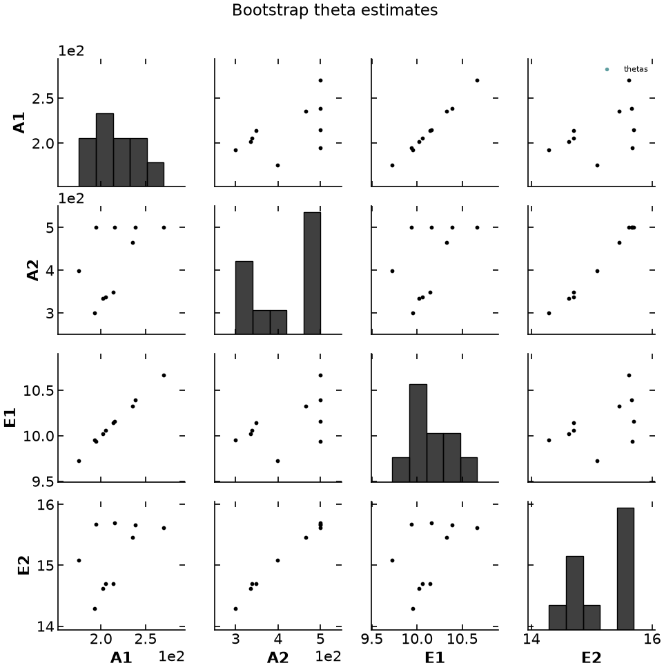
Confidence regions can be plotted around the bootstrap estimates for various distributions with confidence $\alpha$ .

# plot bootstrap parameter estimates with confidence intervals
pyomo.contrib.parmest.graphics.pairwise_plot(
    bootstrap_theta,
    theta,
    0.8,
    ["MVN", "KDE", "Rect"],
    title="Bootstrap theta with confidence regions",
)

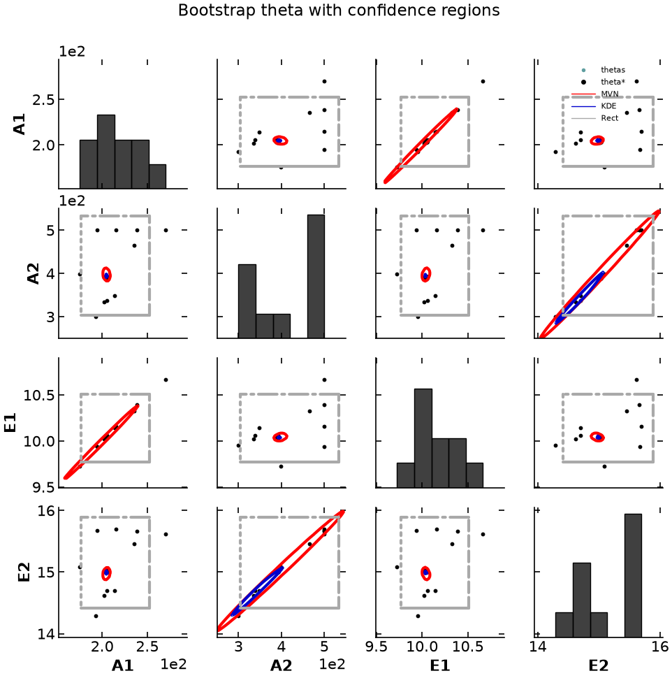
Nonlinear confidence regions¶

The likelihood-ratio test (sometimes called the likelihood-ratio $\chi^2$ test) is a hypothesis test that helps one choose the “best” model between two models link. Basically, the test compares the fit of two models. The null hypothesis is that the first model is the “best” model; It is rejected when the test statistic is large. In other words, if the null hypothesis is rejected, then the second model is a significant improvement over the first model.

In the last part of this notebook, we use the bootstrap parameter estimates to determine the goodness of fit using the likelihood-ratio $\chi^2$ test. More information can be found here.

from itertools import product

### Likelihood ratio test

# generate arrays of parameter values
A1 = np.arange(180.0, 190.0, 1.0)
A2 = np.arange(395.0, 405.0, 1.0)
E1 = np.arange(5.0, 15.0, 1.0)
E2 = np.arange(10.0, 20.0, 1.0)

# format parameter values into a pandas dataframe to be provided as input to calculate
# corresponding objective function values
# theta_vals = pd.DataFrame(list(product(A1, A2, E1, E2)), columns=theta_names)
theta_vals = bootstrap_theta
obj_at_theta = pest.objective_at_theta(theta_vals)
print(obj_at_theta.head())

Ipopt 3.13.2: 

******************************************************************************
This program contains Ipopt, a library for large-scale nonlinear optimization.
 Ipopt is released as open source code under the Eclipse Public License (EPL).
         For more information visit http://projects.coin-or.org/Ipopt

This version of Ipopt was compiled from source code available at
    https://github.com/IDAES/Ipopt as part of the Institute for the Design of
    Advanced Energy Systems Process Systems Engineering Framework (IDAES PSE
    Framework) Copyright (c) 2018-2019. See https://github.com/IDAES/idaes-pse.

This version of Ipopt was compiled using HSL, a collection of Fortran codes
    for large-scale scientific computation.  All technical papers, sales and
    publicity material resulting from use of the HSL codes within IPOPT must
    contain the following acknowledgement:
        HSL, a collection of Fortran codes for large-scale scientific
        computation. See http://www.hsl.rl.ac.uk.
******************************************************************************

This is Ipopt version 3.13.2, running with linear solver ma27.

Number of nonzeros in equality constraint Jacobian...:      640
Number of nonzeros in inequality constraint Jacobian.:        0
Number of nonzeros in Lagrangian Hessian.............:      384

Total number of variables............................:      384
                     variables with only lower bounds:        0
                variables with lower and upper bounds:        0
                     variables with only upper bounds:        0
Total number of equality constraints.................:      384
Total number of inequality constraints...............:        0
        inequality constraints with only lower bounds:        0
   inequality constraints with lower and upper bounds:        0
        inequality constraints with only upper bounds:        0

iter    objective    inf_pr   inf_du lg(mu)  ||d||  lg(rg) alpha_du alpha_pr  ls
   0  1.7195047e+01 2.00e+00 2.50e-01  -1.0 0.00e+00    -  0.00e+00 0.00e+00   0
   1  2.1745504e-01 1.11e-16 3.99e-17  -1.0 2.00e+00    -  1.00e+00 1.00e+00f  1

Number of Iterations....: 1

                                   (scaled)                 (unscaled)
Objective...............:   2.1745503929497820e-01    2.1745503929497820e-01
Dual infeasibility......:   3.4694469519536142e-18    3.4694469519536142e-18
Constraint violation....:   1.1102230246251565e-16    1.1102230246251565e-16
Complementarity.........:   0.0000000000000000e+00    0.0000000000000000e+00
Overall NLP error.......:   1.1102230246251565e-16    1.1102230246251565e-16


Number of objective function evaluations             = 2
Number of objective gradient evaluations             = 2
Number of equality constraint evaluations            = 2
Number of inequality constraint evaluations          = 0
Number of equality constraint Jacobian evaluations   = 2
Number of inequality constraint Jacobian evaluations = 0
Number of Lagrangian Hessian evaluations             = 1
Total CPU secs in IPOPT (w/o function evaluations)   =      0.001
Total CPU secs in NLP function evaluations           =      0.000

EXIT: Optimal Solution Found.

Ipopt 3.13.2: 

******************************************************************************
This program contains Ipopt, a library for large-scale nonlinear optimization.
 Ipopt is released as open source code under the Eclipse Public License (EPL).
         For more information visit http://projects.coin-or.org/Ipopt

This version of Ipopt was compiled from source code available at
    https://github.com/IDAES/Ipopt as part of the Institute for the Design of
    Advanced Energy Systems Process Systems Engineering Framework (IDAES PSE
    Framework) Copyright (c) 2018-2019. See https://github.com/IDAES/idaes-pse.

This version of Ipopt was compiled using HSL, a collection of Fortran codes
    for large-scale scientific computation.  All technical papers, sales and
    publicity material resulting from use of the HSL codes within IPOPT must
    contain the following acknowledgement:
        HSL, a collection of Fortran codes for large-scale scientific
        computation. See http://www.hsl.rl.ac.uk.
******************************************************************************

This is Ipopt version 3.13.2, running with linear solver ma27.

Number of nonzeros in equality constraint Jacobian...:      640
Number of nonzeros in inequality constraint Jacobian.:        0
Number of nonzeros in Lagrangian Hessian.............:      384

Total number of variables............................:      384
                     variables with only lower bounds:        0
                variables with lower and upper bounds:        0
                     variables with only upper bounds:        0
Total number of equality constraints.................:      384
Total number of inequality constraints...............:        0
        inequality constraints with only lower bounds:        0
   inequality constraints with lower and upper bounds:        0
        inequality constraints with only upper bounds:        0

iter    objective    inf_pr   inf_du lg(mu)  ||d||  lg(rg) alpha_du alpha_pr  ls
   0  1.7195047e+01 2.00e+00 2.50e-01  -1.0 0.00e+00    -  0.00e+00 0.00e+00   0
   1  2.1780921e-01 1.11e-16 2.78e-17  -1.0 2.00e+00    -  1.00e+00 1.00e+00f  1

Number of Iterations....: 1

                                   (scaled)                 (unscaled)
Objective...............:   2.1780921357298713e-01    2.1780921357298713e-01
Dual infeasibility......:   3.4694469519536142e-18    3.4694469519536142e-18
Constraint violation....:   1.1102230246251565e-16    1.1102230246251565e-16
Complementarity.........:   0.0000000000000000e+00    0.0000000000000000e+00
Overall NLP error.......:   1.1102230246251565e-16    1.1102230246251565e-16


Number of objective function evaluations             = 2
Number of objective gradient evaluations             = 2
Number of equality constraint evaluations            = 2
Number of inequality constraint evaluations          = 0
Number of equality constraint Jacobian evaluations   = 2
Number of inequality constraint Jacobian evaluations = 0
Number of Lagrangian Hessian evaluations             = 1
Total CPU secs in IPOPT (w/o function evaluations)   =      0.001
Total CPU secs in NLP function evaluations           =      0.000

EXIT: Optimal Solution Found.

Ipopt 3.13.2: 

******************************************************************************
This program contains Ipopt, a library for large-scale nonlinear optimization.
 Ipopt is released as open source code under the Eclipse Public License (EPL).
         For more information visit http://projects.coin-or.org/Ipopt

This version of Ipopt was compiled from source code available at
    https://github.com/IDAES/Ipopt as part of the Institute for the Design of
    Advanced Energy Systems Process Systems Engineering Framework (IDAES PSE
    Framework) Copyright (c) 2018-2019. See https://github.com/IDAES/idaes-pse.

This version of Ipopt was compiled using HSL, a collection of Fortran codes
    for large-scale scientific computation.  All technical papers, sales and
    publicity material resulting from use of the HSL codes within IPOPT must
    contain the following acknowledgement:
        HSL, a collection of Fortran codes for large-scale scientific
        computation. See http://www.hsl.rl.ac.uk.
******************************************************************************

This is Ipopt version 3.13.2, running with linear solver ma27.

Number of nonzeros in equality constraint Jacobian...:      640
Number of nonzeros in inequality constraint Jacobian.:        0
Number of nonzeros in Lagrangian Hessian.............:      384

Total number of variables............................:      384
                     variables with only lower bounds:        0
                variables with lower and upper bounds:        0
                     variables with only upper bounds:        0
Total number of equality constraints.................:      384
Total number of inequality constraints...............:        0
        inequality constraints with only lower bounds:        0
   inequality constraints with lower and upper bounds:        0
        inequality constraints with only upper bounds:        0

iter    objective    inf_pr   inf_du lg(mu)  ||d||  lg(rg) alpha_du alpha_pr  ls
   0  1.7195047e+01 2.00e+00 2.50e-01  -1.0 0.00e+00    -  0.00e+00 0.00e+00   0
   1  2.1850598e-01 1.11e-16 3.99e-17  -1.0 2.00e+00    -  1.00e+00 1.00e+00f  1

Number of Iterations....: 1

                                   (scaled)                 (unscaled)
Objective...............:   2.1850598156002982e-01    2.1850598156002982e-01
Dual infeasibility......:   3.4694469519536142e-18    3.4694469519536142e-18
Constraint violation....:   1.1102230246251565e-16    1.1102230246251565e-16
Complementarity.........:   0.0000000000000000e+00    0.0000000000000000e+00
Overall NLP error.......:   1.1102230246251565e-16    1.1102230246251565e-16


Number of objective function evaluations             = 2
Number of objective gradient evaluations             = 2
Number of equality constraint evaluations            = 2
Number of inequality constraint evaluations          = 0
Number of equality constraint Jacobian evaluations   = 2
Number of inequality constraint Jacobian evaluations = 0
Number of Lagrangian Hessian evaluations             = 1
Total CPU secs in IPOPT (w/o function evaluations)   =      0.001
Total CPU secs in NLP function evaluations           =      0.000

EXIT: Optimal Solution Found.

Ipopt 3.13.2: 

******************************************************************************
This program contains Ipopt, a library for large-scale nonlinear optimization.
 Ipopt is released as open source code under the Eclipse Public License (EPL).
         For more information visit http://projects.coin-or.org/Ipopt

This version of Ipopt was compiled from source code available at
    https://github.com/IDAES/Ipopt as part of the Institute for the Design of
    Advanced Energy Systems Process Systems Engineering Framework (IDAES PSE
    Framework) Copyright (c) 2018-2019. See https://github.com/IDAES/idaes-pse.

This version of Ipopt was compiled using HSL, a collection of Fortran codes
    for large-scale scientific computation.  All technical papers, sales and
    publicity material resulting from use of the HSL codes within IPOPT must
    contain the following acknowledgement:
        HSL, a collection of Fortran codes for large-scale scientific
        computation. See http://www.hsl.rl.ac.uk.
******************************************************************************

This is Ipopt version 3.13.2, running with linear solver ma27.

Number of nonzeros in equality constraint Jacobian...:      640
Number of nonzeros in inequality constraint Jacobian.:        0
Number of nonzeros in Lagrangian Hessian.............:      384

Total number of variables............................:      384
                     variables with only lower bounds:        0
                variables with lower and upper bounds:        0
                     variables with only upper bounds:        0
Total number of equality constraints.................:      384
Total number of inequality constraints...............:        0
        inequality constraints with only lower bounds:        0
   inequality constraints with lower and upper bounds:        0
        inequality constraints with only upper bounds:        0

iter    objective    inf_pr   inf_du lg(mu)  ||d||  lg(rg) alpha_du alpha_pr  ls
   0  1.7195047e+01 2.00e+00 2.50e-01  -1.0 0.00e+00    -  0.00e+00 0.00e+00   0
   1  2.1865678e-01 1.11e-16 3.82e-17  -1.0 2.00e+00    -  1.00e+00 1.00e+00f  1

Number of Iterations....: 1

                                   (scaled)                 (unscaled)
Objective...............:   2.1865678205281217e-01    2.1865678205281217e-01
Dual infeasibility......:   3.4694469519536142e-18    3.4694469519536142e-18
Constraint violation....:   1.1102230246251565e-16    1.1102230246251565e-16
Complementarity.........:   0.0000000000000000e+00    0.0000000000000000e+00
Overall NLP error.......:   1.1102230246251565e-16    1.1102230246251565e-16


Number of objective function evaluations             = 2
Number of objective gradient evaluations             = 2
Number of equality constraint evaluations            = 2
Number of inequality constraint evaluations          = 0
Number of equality constraint Jacobian evaluations   = 2
Number of inequality constraint Jacobian evaluations = 0
Number of Lagrangian Hessian evaluations             = 1
Total CPU secs in IPOPT (w/o function evaluations)   =      0.001
Total CPU secs in NLP function evaluations           =      0.000

EXIT: Optimal Solution Found.

Ipopt 3.13.2: 

******************************************************************************
This program contains Ipopt, a library for large-scale nonlinear optimization.
 Ipopt is released as open source code under the Eclipse Public License (EPL).
         For more information visit http://projects.coin-or.org/Ipopt

This version of Ipopt was compiled from source code available at
    https://github.com/IDAES/Ipopt as part of the Institute for the Design of
    Advanced Energy Systems Process Systems Engineering Framework (IDAES PSE
    Framework) Copyright (c) 2018-2019. See https://github.com/IDAES/idaes-pse.

This version of Ipopt was compiled using HSL, a collection of Fortran codes
    for large-scale scientific computation.  All technical papers, sales and
    publicity material resulting from use of the HSL codes within IPOPT must
    contain the following acknowledgement:
        HSL, a collection of Fortran codes for large-scale scientific
        computation. See http://www.hsl.rl.ac.uk.
******************************************************************************

This is Ipopt version 3.13.2, running with linear solver ma27.

Number of nonzeros in equality constraint Jacobian...:      640
Number of nonzeros in inequality constraint Jacobian.:        0
Number of nonzeros in Lagrangian Hessian.............:      384

Total number of variables............................:      384
                     variables with only lower bounds:        0
                variables with lower and upper bounds:        0
                     variables with only upper bounds:        0
Total number of equality constraints.................:      384
Total number of inequality constraints...............:        0
        inequality constraints with only lower bounds:        0
   inequality constraints with lower and upper bounds:        0
        inequality constraints with only upper bounds:        0

iter    objective    inf_pr   inf_du lg(mu)  ||d||  lg(rg) alpha_du alpha_pr  ls
   0  1.7195047e+01 2.00e+00 2.50e-01  -1.0 0.00e+00    -  0.00e+00 0.00e+00   0
   1  2.1971783e-01 1.11e-16 3.82e-17  -1.0 2.00e+00    -  1.00e+00 1.00e+00f  1

Number of Iterations....: 1

                                   (scaled)                 (unscaled)
Objective...............:   2.1971782743526694e-01    2.1971782743526694e-01
Dual infeasibility......:   3.4694469519536142e-18    3.4694469519536142e-18
Constraint violation....:   1.1102230246251565e-16    1.1102230246251565e-16
Complementarity.........:   0.0000000000000000e+00    0.0000000000000000e+00
Overall NLP error.......:   1.1102230246251565e-16    1.1102230246251565e-16


Number of objective function evaluations             = 2
Number of objective gradient evaluations             = 2
Number of equality constraint evaluations            = 2
Number of inequality constraint evaluations          = 0
Number of equality constraint Jacobian evaluations   = 2
Number of inequality constraint Jacobian evaluations = 0
Number of Lagrangian Hessian evaluations             = 1
Total CPU secs in IPOPT (w/o function evaluations)   =      0.001
Total CPU secs in NLP function evaluations           =      0.000

EXIT: Optimal Solution Found.

Ipopt 3.13.2: 

******************************************************************************
This program contains Ipopt, a library for large-scale nonlinear optimization.
 Ipopt is released as open source code under the Eclipse Public License (EPL).
         For more information visit http://projects.coin-or.org/Ipopt

This version of Ipopt was compiled from source code available at
    https://github.com/IDAES/Ipopt as part of the Institute for the Design of
    Advanced Energy Systems Process Systems Engineering Framework (IDAES PSE
    Framework) Copyright (c) 2018-2019. See https://github.com/IDAES/idaes-pse.

This version of Ipopt was compiled using HSL, a collection of Fortran codes
    for large-scale scientific computation.  All technical papers, sales and
    publicity material resulting from use of the HSL codes within IPOPT must
    contain the following acknowledgement:
        HSL, a collection of Fortran codes for large-scale scientific
        computation. See http://www.hsl.rl.ac.uk.
******************************************************************************

This is Ipopt version 3.13.2, running with linear solver ma27.

Number of nonzeros in equality constraint Jacobian...:      640
Number of nonzeros in inequality constraint Jacobian.:        0
Number of nonzeros in Lagrangian Hessian.............:      384

Total number of variables............................:      384
                     variables with only lower bounds:        0
                variables with lower and upper bounds:        0
                     variables with only upper bounds:        0
Total number of equality constraints.................:      384
Total number of inequality constraints...............:        0
        inequality constraints with only lower bounds:        0
   inequality constraints with lower and upper bounds:        0
        inequality constraints with only upper bounds:        0

iter    objective    inf_pr   inf_du lg(mu)  ||d||  lg(rg) alpha_du alpha_pr  ls
   0  1.7195047e+01 2.00e+00 2.50e-01  -1.0 0.00e+00    -  0.00e+00 0.00e+00   0
   1  2.1854819e-01 1.11e-16 3.82e-17  -1.0 2.00e+00    -  1.00e+00 1.00e+00f  1

Number of Iterations....: 1

                                   (scaled)                 (unscaled)
Objective...............:   2.1854819378354320e-01    2.1854819378354320e-01
Dual infeasibility......:   3.4694469519536142e-18    3.4694469519536142e-18
Constraint violation....:   1.1102230246251565e-16    1.1102230246251565e-16
Complementarity.........:   0.0000000000000000e+00    0.0000000000000000e+00
Overall NLP error.......:   1.1102230246251565e-16    1.1102230246251565e-16


Number of objective function evaluations             = 2
Number of objective gradient evaluations             = 2
Number of equality constraint evaluations            = 2
Number of inequality constraint evaluations          = 0
Number of equality constraint Jacobian evaluations   = 2
Number of inequality constraint Jacobian evaluations = 0
Number of Lagrangian Hessian evaluations             = 1
Total CPU secs in IPOPT (w/o function evaluations)   =      0.000
Total CPU secs in NLP function evaluations           =      0.000

EXIT: Optimal Solution Found.

Ipopt 3.13.2: 

******************************************************************************
This program contains Ipopt, a library for large-scale nonlinear optimization.
 Ipopt is released as open source code under the Eclipse Public License (EPL).
         For more information visit http://projects.coin-or.org/Ipopt

This version of Ipopt was compiled from source code available at
    https://github.com/IDAES/Ipopt as part of the Institute for the Design of
    Advanced Energy Systems Process Systems Engineering Framework (IDAES PSE
    Framework) Copyright (c) 2018-2019. See https://github.com/IDAES/idaes-pse.

This version of Ipopt was compiled using HSL, a collection of Fortran codes
    for large-scale scientific computation.  All technical papers, sales and
    publicity material resulting from use of the HSL codes within IPOPT must
    contain the following acknowledgement:
        HSL, a collection of Fortran codes for large-scale scientific
        computation. See http://www.hsl.rl.ac.uk.
******************************************************************************

This is Ipopt version 3.13.2, running with linear solver ma27.

Number of nonzeros in equality constraint Jacobian...:      640
Number of nonzeros in inequality constraint Jacobian.:        0
Number of nonzeros in Lagrangian Hessian.............:      384

Total number of variables............................:      384
                     variables with only lower bounds:        0
                variables with lower and upper bounds:        0
                     variables with only upper bounds:        0
Total number of equality constraints.................:      384
Total number of inequality constraints...............:        0
        inequality constraints with only lower bounds:        0
   inequality constraints with lower and upper bounds:        0
        inequality constraints with only upper bounds:        0

iter    objective    inf_pr   inf_du lg(mu)  ||d||  lg(rg) alpha_du alpha_pr  ls
   0  1.7195047e+01 2.00e+00 2.50e-01  -1.0 0.00e+00    -  0.00e+00 0.00e+00   0
   1  2.1887464e-01 1.11e-16 3.47e-17  -1.0 2.00e+00    -  1.00e+00 1.00e+00f  1

Number of Iterations....: 1

                                   (scaled)                 (unscaled)
Objective...............:   2.1887463798800386e-01    2.1887463798800386e-01
Dual infeasibility......:   3.4694469519536142e-18    3.4694469519536142e-18
Constraint violation....:   1.1102230246251565e-16    1.1102230246251565e-16
Complementarity.........:   0.0000000000000000e+00    0.0000000000000000e+00
Overall NLP error.......:   1.1102230246251565e-16    1.1102230246251565e-16


Number of objective function evaluations             = 2
Number of objective gradient evaluations             = 2
Number of equality constraint evaluations            = 2
Number of inequality constraint evaluations          = 0
Number of equality constraint Jacobian evaluations   = 2
Number of inequality constraint Jacobian evaluations = 0
Number of Lagrangian Hessian evaluations             = 1
Total CPU secs in IPOPT (w/o function evaluations)   =      0.001
Total CPU secs in NLP function evaluations           =      0.000

EXIT: Optimal Solution Found.

Ipopt 3.13.2: 

******************************************************************************
This program contains Ipopt, a library for large-scale nonlinear optimization.
 Ipopt is released as open source code under the Eclipse Public License (EPL).
         For more information visit http://projects.coin-or.org/Ipopt

This version of Ipopt was compiled from source code available at
    https://github.com/IDAES/Ipopt as part of the Institute for the Design of
    Advanced Energy Systems Process Systems Engineering Framework (IDAES PSE
    Framework) Copyright (c) 2018-2019. See https://github.com/IDAES/idaes-pse.

This version of Ipopt was compiled using HSL, a collection of Fortran codes
    for large-scale scientific computation.  All technical papers, sales and
    publicity material resulting from use of the HSL codes within IPOPT must
    contain the following acknowledgement:
        HSL, a collection of Fortran codes for large-scale scientific
        computation. See http://www.hsl.rl.ac.uk.
******************************************************************************

This is Ipopt version 3.13.2, running with linear solver ma27.

Number of nonzeros in equality constraint Jacobian...:      640
Number of nonzeros in inequality constraint Jacobian.:        0
Number of nonzeros in Lagrangian Hessian.............:      384

Total number of variables............................:      384
                     variables with only lower bounds:        0
                variables with lower and upper bounds:        0
                     variables with only upper bounds:        0
Total number of equality constraints.................:      384
Total number of inequality constraints...............:        0
        inequality constraints with only lower bounds:        0
   inequality constraints with lower and upper bounds:        0
        inequality constraints with only upper bounds:        0

iter    objective    inf_pr   inf_du lg(mu)  ||d||  lg(rg) alpha_du alpha_pr  ls
   0  1.7195047e+01 2.00e+00 2.50e-01  -1.0 0.00e+00    -  0.00e+00 0.00e+00   0
   1  2.2065040e-01 1.11e-16 3.82e-17  -1.0 2.00e+00    -  1.00e+00 1.00e+00f  1

Number of Iterations....: 1

                                   (scaled)                 (unscaled)
Objective...............:   2.2065039827490601e-01    2.2065039827490601e-01
Dual infeasibility......:   3.4694469519536142e-18    3.4694469519536142e-18
Constraint violation....:   1.1102230246251565e-16    1.1102230246251565e-16
Complementarity.........:   0.0000000000000000e+00    0.0000000000000000e+00
Overall NLP error.......:   1.1102230246251565e-16    1.1102230246251565e-16


Number of objective function evaluations             = 2
Number of objective gradient evaluations             = 2
Number of equality constraint evaluations            = 2
Number of inequality constraint evaluations          = 0
Number of equality constraint Jacobian evaluations   = 2
Number of inequality constraint Jacobian evaluations = 0
Number of Lagrangian Hessian evaluations             = 1
Total CPU secs in IPOPT (w/o function evaluations)   =      0.001
Total CPU secs in NLP function evaluations           =      0.000

EXIT: Optimal Solution Found.

Ipopt 3.13.2: 

******************************************************************************
This program contains Ipopt, a library for large-scale nonlinear optimization.
 Ipopt is released as open source code under the Eclipse Public License (EPL).
         For more information visit http://projects.coin-or.org/Ipopt

This version of Ipopt was compiled from source code available at
    https://github.com/IDAES/Ipopt as part of the Institute for the Design of
    Advanced Energy Systems Process Systems Engineering Framework (IDAES PSE
    Framework) Copyright (c) 2018-2019. See https://github.com/IDAES/idaes-pse.

This version of Ipopt was compiled using HSL, a collection of Fortran codes
    for large-scale scientific computation.  All technical papers, sales and
    publicity material resulting from use of the HSL codes within IPOPT must
    contain the following acknowledgement:
        HSL, a collection of Fortran codes for large-scale scientific
        computation. See http://www.hsl.rl.ac.uk.
******************************************************************************

This is Ipopt version 3.13.2, running with linear solver ma27.

Number of nonzeros in equality constraint Jacobian...:      640
Number of nonzeros in inequality constraint Jacobian.:        0
Number of nonzeros in Lagrangian Hessian.............:      384

Total number of variables............................:      384
                     variables with only lower bounds:        0
                variables with lower and upper bounds:        0
                     variables with only upper bounds:        0
Total number of equality constraints.................:      384
Total number of inequality constraints...............:        0
        inequality constraints with only lower bounds:        0
   inequality constraints with lower and upper bounds:        0
        inequality constraints with only upper bounds:        0

iter    objective    inf_pr   inf_du lg(mu)  ||d||  lg(rg) alpha_du alpha_pr  ls
   0  1.7195047e+01 2.00e+00 2.50e-01  -1.0 0.00e+00    -  0.00e+00 0.00e+00   0
   1  2.2512139e-01 1.11e-16 2.78e-17  -1.0 2.00e+00    -  1.00e+00 1.00e+00f  1

Number of Iterations....: 1

                                   (scaled)                 (unscaled)
Objective...............:   2.2512138716553287e-01    2.2512138716553287e-01
Dual infeasibility......:   3.4694469519536142e-18    3.4694469519536142e-18
Constraint violation....:   1.1102230246251565e-16    1.1102230246251565e-16
Complementarity.........:   0.0000000000000000e+00    0.0000000000000000e+00
Overall NLP error.......:   1.1102230246251565e-16    1.1102230246251565e-16


Number of objective function evaluations             = 2
Number of objective gradient evaluations             = 2
Number of equality constraint evaluations            = 2
Number of inequality constraint evaluations          = 0
Number of equality constraint Jacobian evaluations   = 2
Number of inequality constraint Jacobian evaluations = 0
Number of Lagrangian Hessian evaluations             = 1
Total CPU secs in IPOPT (w/o function evaluations)   =      0.000
Total CPU secs in NLP function evaluations           =      0.000

EXIT: Optimal Solution Found.

Ipopt 3.13.2: 

******************************************************************************
This program contains Ipopt, a library for large-scale nonlinear optimization.
 Ipopt is released as open source code under the Eclipse Public License (EPL).
         For more information visit http://projects.coin-or.org/Ipopt

This version of Ipopt was compiled from source code available at
    https://github.com/IDAES/Ipopt as part of the Institute for the Design of
    Advanced Energy Systems Process Systems Engineering Framework (IDAES PSE
    Framework) Copyright (c) 2018-2019. See https://github.com/IDAES/idaes-pse.

This version of Ipopt was compiled using HSL, a collection of Fortran codes
    for large-scale scientific computation.  All technical papers, sales and
    publicity material resulting from use of the HSL codes within IPOPT must
    contain the following acknowledgement:
        HSL, a collection of Fortran codes for large-scale scientific
        computation. See http://www.hsl.rl.ac.uk.
******************************************************************************

This is Ipopt version 3.13.2, running with linear solver ma27.

Number of nonzeros in equality constraint Jacobian...:      640
Number of nonzeros in inequality constraint Jacobian.:        0
Number of nonzeros in Lagrangian Hessian.............:      384

Total number of variables............................:      384
                     variables with only lower bounds:        0
                variables with lower and upper bounds:        0
                     variables with only upper bounds:        0
Total number of equality constraints.................:      384
Total number of inequality constraints...............:        0
        inequality constraints with only lower bounds:        0
   inequality constraints with lower and upper bounds:        0
        inequality constraints with only upper bounds:        0

iter    objective    inf_pr   inf_du lg(mu)  ||d||  lg(rg) alpha_du alpha_pr  ls
   0  1.7195047e+01 2.00e+00 2.50e-01  -1.0 0.00e+00    -  0.00e+00 0.00e+00   0
   1  2.2045496e-01 1.11e-16 3.82e-17  -1.0 2.00e+00    -  1.00e+00 1.00e+00f  1

Number of Iterations....: 1

                                   (scaled)                 (unscaled)
Objective...............:   2.2045496207202267e-01    2.2045496207202267e-01
Dual infeasibility......:   3.4694469519536142e-18    3.4694469519536142e-18
Constraint violation....:   1.1102230246251565e-16    1.1102230246251565e-16
Complementarity.........:   0.0000000000000000e+00    0.0000000000000000e+00
Overall NLP error.......:   1.1102230246251565e-16    1.1102230246251565e-16


Number of objective function evaluations             = 2
Number of objective gradient evaluations             = 2
Number of equality constraint evaluations            = 2
Number of inequality constraint evaluations          = 0
Number of equality constraint Jacobian evaluations   = 2
Number of inequality constraint Jacobian evaluations = 0
Number of Lagrangian Hessian evaluations             = 1
Total CPU secs in IPOPT (w/o function evaluations)   =      0.001
Total CPU secs in NLP function evaluations           =      0.000

EXIT: Optimal Solution Found.

           A1          A2         E1         E2       obj
0  214.006137  348.422627  10.145437  14.702458  0.217455
1  202.042787  334.816774  10.020204  14.615005  0.217809
2  194.760940  499.988962   9.937919  15.673948  0.218506
3  215.170330  499.988460  10.162064  15.698181  0.218657
4  192.739676  300.015132   9.950830  14.294222  0.219718

LR = pest.likelihood_ratio_test(obj_at_theta, obj, [0.8, 0.85, 0.9, 0.95])
print(LR.head())

           A1          A2         E1         E2       obj   0.8  0.85   0.9  \
0  214.006137  348.422627  10.145437  14.702458  0.217455  True  True  True   
1  202.042787  334.816774  10.020204  14.615005  0.217809  True  True  True   
2  194.760940  499.988962   9.937919  15.673948  0.218506  True  True  True   
3  215.170330  499.988460  10.162064  15.698181  0.218657  True  True  True   
4  192.739676  300.015132   9.950830  14.294222  0.219718  True  True  True   

   0.95  
0  True  
1  True  
2  True  
3  True  
4  True

The likelihood ratio test results with confidence $\alpha$ can be visualized as follows:

pyomo.contrib.parmest.graphics.pairwise_plot(
    LR, theta, 0.8, title="LR results within 80% confidence region"
)

Objective contour plot for A1 A2 slice failed
Objective contour plot for A1 E1 slice failed
Objective contour plot for A2 E1 slice failed
Objective contour plot for A1 E2 slice failed
Objective contour plot for A2 E2 slice failed
Objective contour plot for E1 E2 slice failed
Objective contour plot for A2 A1 slice failed
Objective contour plot for E1 A1 slice failed
Objective contour plot for E2 A1 slice failed
Objective contour plot for E1 A2 slice failed
Objective contour plot for E2 A2 slice failed
Objective contour plot for E2 E1 slice failed

References¶

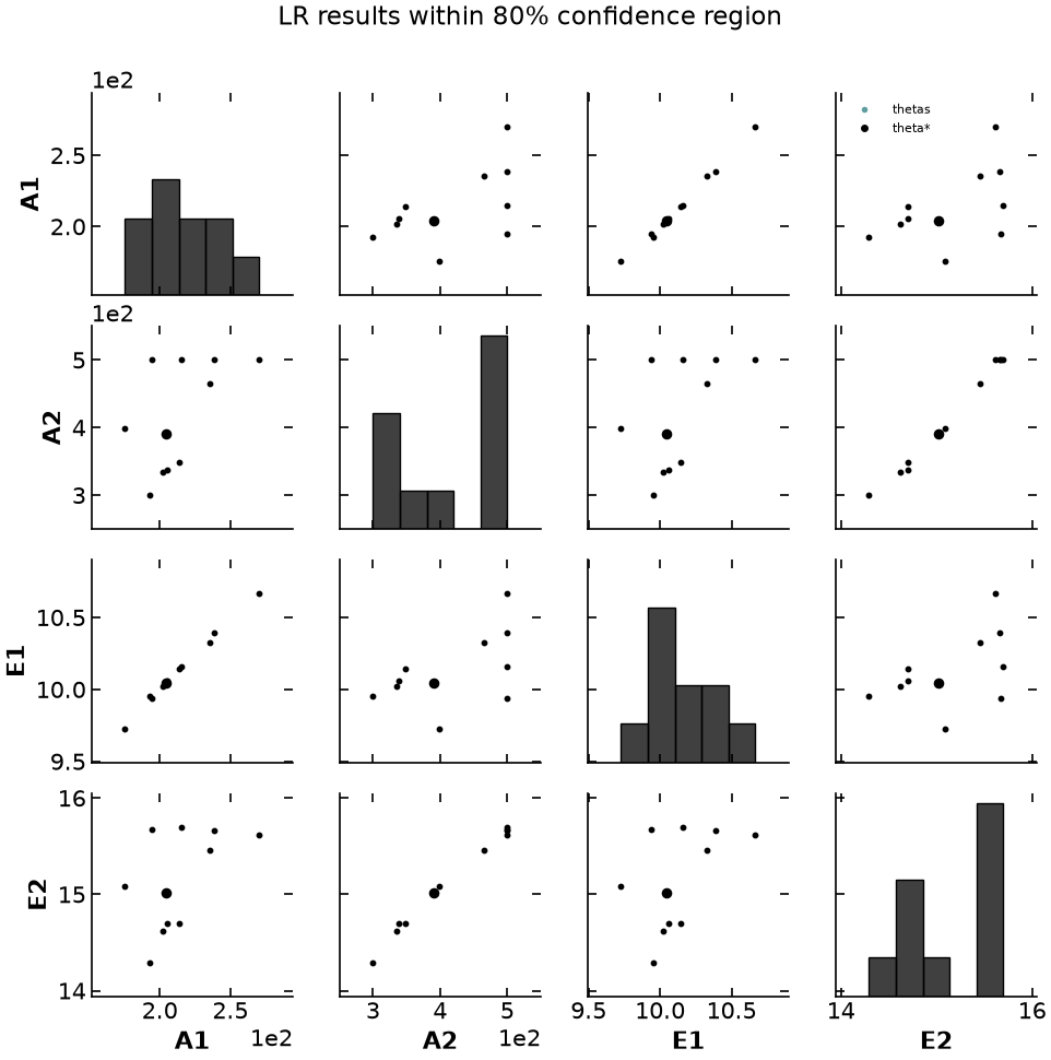
Chen, W., & Biegler, L. T. (2020). Reduced Hessian based parameter selection and estimation with simultaneous collocation approach. AIChE Journal, 66(7). 10.1002/aic.16242

What is parameter estimation?¶

What is parmest?¶

Example: Reaction Kinetics¶

Batch Reactor¶

Experimental Data¶

Pyomo model¶

Parameter estimation with a single dataset¶

Parameter estimation with multiple datasets¶

Generate Experiment list¶

Parameter estimation with parmest¶

Plotting fitted model simulation with ‘experimental’ data¶

Using parmest with pyomo.dae¶

Parameter estimation with parmest¶

Plotting fitted model simulation with ‘experimental’ data¶

Local uncertainty analysis¶

Covariance matrix¶

Parameter identifiability¶

Bootstrap resampling¶

Nonlinear confidence regions¶

What is `parmest`?¶

Using `parmest` with `pyomo.dae`¶