How Much Does a Better Forecast Help? - Optimization for Decision Science

This companion revisits battery arbitrage with uncertain prices. At each decision hour, we build scenarios only from older prices, implement one action, observe the realized price, and replan.

The notebook separates three questions:

What is the value of perfect information at one forecast origin?
Does modeling forecast uncertainty improve the first action?
How do the policies perform out of sample in a rolling backtest?

Learning goals¶

Put shared first-stage decisions on the root model and recourse on scenario Blocks.
Distinguish a two-stage approximation from a multistage scenario tree.
Compute RP, EEV, WS, VSS, and EVPI with the profit convention.
Prevent simultaneous charging and discharging, including at negative prices.
Compare expected-value, stochastic, risk-averse, and perfect-forecast policies.

# Install course dependencies before importing Pyomo on Colab.
import sys

if "google.colab" in sys.modules:
    !wget "https://raw.githubusercontent.com/ndcbe/optimization/main/notebooks/helper.py"
    import helper

    helper.easy_install()
else:
    sys.path.insert(0, "../")
    import helper

helper.set_plotting_style()

import matplotlib.pyplot as plt
import numpy as np
import pandas as pd
import pyomo.environ as pyo

SOLVER = pyo.SolverFactory("appsi_highs")
assert SOLVER.available(
    exception_flag=False
), "Install HiGHS before running this notebook."

Data and information pattern¶

The repository supplies a historical CAISO day-ahead price series in Prices_DAM_ALTA2G_7_B1.csv. The teaching model treats each entry as one hour. This is an illustrative sequential-information experiment, not a reconstruction of day-ahead auction timing: in an actual day-ahead schedule, the next day’s clearing prices are not revealed one hour at a time.

At decision hour $t$ :

the seven scenarios are 24-hour windows beginning at the same hour on the previous seven days;
every scenario ends at or before $t$ ;
the realized window beginning at $t$ is reserved for evaluation; and
an oracle policy may use that window only as an unattainable benchmark.

This historical ensemble is transparent, not a claim of forecasting state of the art. See CAISO’s market description for actual day-ahead timing.

prices = pd.read_csv("https://raw.githubusercontent.com/ndcbe/optimization/main/notebooks/data/Prices_DAM_ALTA2G_7_B1.csv", names=["price"])[
    "price"
].to_numpy(float)

HORIZON = 24
N_SCENARIOS = 7
FIRST_BACKTEST_HOUR = 678
BACKTEST_HOURS = 48

assert FIRST_BACKTEST_HOUR >= N_SCENARIOS * 24
assert FIRST_BACKTEST_HOUR + BACKTEST_HOURS + HORIZON <= len(prices)


def backcast_scenarios(
    price_history, decision_hour, horizon=HORIZON, n_scenarios=N_SCENARIOS
):
    # Aligned historical price paths available by decision_hour.
    starts = [decision_hour - 24 * day for day in range(1, n_scenarios + 1)]
    scenarios = np.vstack([price_history[start : start + horizon] for start in starts])
    assert max(start + horizon for start in starts) <= decision_hour
    return scenarios


scenarios = backcast_scenarios(prices, FIRST_BACKTEST_HOUR)
# Small multiples keep no more than three historical paths on each axes.
fig, axes = plt.subplots(3, 1, figsize=(9, 9), sharex=True, layout="constrained")
for group, ax in enumerate(axes):
    for k in range(group * 3, min((group + 1) * 3, len(scenarios))):
        ax.plot(
            scenarios[k],
            linestyle=["-", "--", ":"][k % 3],
            label=f"{k + 1} day(s) earlier",
        )
    ax.plot(
        scenarios.mean(axis=0), color="black", linestyle="-.", label="Mean of 7 paths"
    )
    ax.set_ylabel("Price [$/MWh]")
    ax.legend(fontsize=10, ncol=2)
axes[-1].set_xlabel("Hours ahead")
plt.show()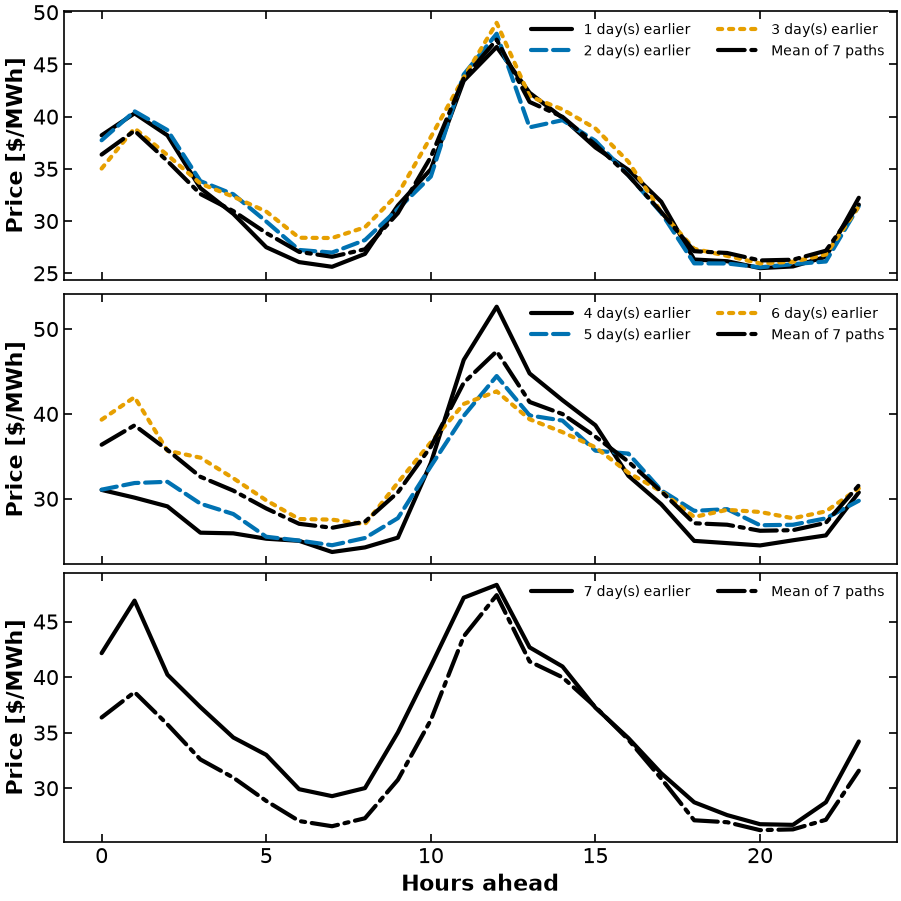

Two-stage scenario-block model¶

Battery assumptions:

1-hour time steps;
1 MW charge and discharge limits;
4 MWh energy capacity;
92% one-way efficiency; and
terminal energy equals initial energy over each planning horizon.

The root variables are the action implemented now. Every scenario block contains later recourse decisions and its own price path. Only the first action is nonanticipative, so this is a two-stage approximation: after hour 0, each scenario acts as though its entire path were revealed. A true multistage model would need a scenario tree and nonanticipativity at every shared history.

Binary operating modes prevent simultaneous charge and discharge. This matters when prices are negative: without the modes, artificial cycling losses can become profitable.

POWER_CAPACITY = 1.0  # MW
ENERGY_CAPACITY = 4.0  # MWh
EFFICIENCY = 0.92


def build_battery_model(
    price_scenarios,
    initial_energy,
    terminal_energy=None,
    risk_weight=0.0,
    cvar_confidence=0.90,
):
    """Build a two-stage MILP with one-hour steps and equal scenario weights.

    Power is MW, energy MWh, prices dollars/MWh; all profit terms are dollars.
    Only hour zero is shared. Later actions anticipate each full scenario path.
    Args: price_scenarios [$/MWh], initial/terminal energy [MWh],
        risk_weight [0, 1], and cvar_confidence (0, 1).
    Returns: a fresh Pyomo ConcreteModel with a profit-maximizing objective.
    """
    if not 0 <= risk_weight <= 1 or not 0 < cvar_confidence < 1:
        raise ValueError("Require weight in [0, 1] and confidence in (0, 1)")
    price_scenarios = np.asarray(price_scenarios, dtype=float)
    n_scenarios, horizon = price_scenarios.shape
    terminal_energy = initial_energy if terminal_energy is None else terminal_energy

    m = pyo.ConcreteModel()
    m.S = pyo.RangeSet(0, n_scenarios - 1)
    m.T = pyo.RangeSet(0, horizon - 1)
    m.probability = pyo.Param(m.S, initialize=1 / n_scenarios)

    # Shared first-stage action.
    m.first_charge = pyo.Var(bounds=(0, POWER_CAPACITY))
    m.first_discharge = pyo.Var(bounds=(0, POWER_CAPACITY))
    m.first_mode = pyo.Var(domain=pyo.Binary)
    m.first_charge_limit = pyo.Constraint(
        expr=m.first_charge <= POWER_CAPACITY * m.first_mode
    )
    m.first_discharge_limit = pyo.Constraint(
        expr=m.first_discharge <= POWER_CAPACITY * (1 - m.first_mode)
    )

    def scenario_rule(block, scenario):
        block.price = pyo.Param(
            m.T, initialize=lambda block, hour: price_scenarios[scenario, hour]
        )
        block.charge = pyo.Var(m.T, domain=pyo.NonNegativeReals)
        block.discharge = pyo.Var(m.T, domain=pyo.NonNegativeReals)
        block.energy = pyo.Var(m.T, bounds=(0, ENERGY_CAPACITY))
        block.mode = pyo.Var(m.T, domain=pyo.Binary)

        @block.Constraint(m.T)
        def charge_limit(b, hour):
            return b.charge[hour] <= POWER_CAPACITY * b.mode[hour]

        @block.Constraint(m.T)
        def discharge_limit(b, hour):
            return b.discharge[hour] <= POWER_CAPACITY * (1 - b.mode[hour])

        # A one-hour step converts MW to MWh; efficiency acts on each flow.
        @block.Constraint(m.T)
        def energy_balance(b, hour):
            previous = initial_energy if hour == 0 else b.energy[hour - 1]
            return b.energy[hour] == (
                previous + EFFICIENCY * b.charge[hour] - b.discharge[hour] / EFFICIENCY
            )

        block.terminal = pyo.Constraint(
            expr=block.energy[horizon - 1] == terminal_energy
        )
        # Linking every scenario to root actions enforces nonanticipativity.
        block.link_charge = pyo.Constraint(expr=block.charge[0] == m.first_charge)
        block.link_discharge = pyo.Constraint(
            expr=block.discharge[0] == m.first_discharge
        )
        block.link_mode = pyo.Constraint(expr=block.mode[0] == m.first_mode)
        block.profit = pyo.Expression(
            expr=sum(
                block.price[hour] * (block.discharge[hour] - block.charge[hour])
                for hour in m.T
            )
        )

    m.scenario = pyo.Block(m.S, rule=scenario_rule)
    m.expected_profit = pyo.Expression(
        expr=sum(m.probability[s] * m.scenario[s].profit for s in m.S)
    )

    # Lower-tail PROFIT CVaR is minus upper-tail CVaR of negative profit.
    if risk_weight > 0:
        # An optimal threshold may be nonunique; do not call it unique VaR.
        m.profit_var = pyo.Var()
        for s in m.S:
            block = m.scenario[s]
            block.shortfall = pyo.Var(domain=pyo.NonNegativeReals)
            block.shortfall_constraint = pyo.Constraint(
                expr=block.shortfall >= m.profit_var - block.profit
            )
        m.lower_tail_cvar = pyo.Expression(
            expr=m.profit_var
            - sum(m.probability[s] * m.scenario[s].shortfall for s in m.S)
            / (1 - cvar_confidence)
        )
        m.objective = pyo.Objective(
            expr=(1 - risk_weight) * m.expected_profit
            + risk_weight * m.lower_tail_cvar,
            sense=pyo.maximize,
        )
    else:
        m.objective = pyo.Objective(expr=m.expected_profit, sense=pyo.maximize)
    return m


def solve(model):
    result = SOLVER.solve(model)
    assert pyo.check_optimal_termination(result), result.solver.termination_condition
    return model


def first_action(model):
    return (
        float(pyo.value(model.first_charge)),
        float(pyo.value(model.first_discharge)),
    )

Value of information at one forecast origin¶

Using the profit convention:

RP solves the two-stage recourse problem;
EEV fixes the expected-value model’s first action, then evaluates its recourse;
WS averages independent perfect-information solutions;
$\mathrm{VSS}=RP-EEV$ ; and
$\mathrm{EVPI}=WS-RP$ .

For a maximization problem, $WS\ge RP\ge EEV$ up to solver tolerance. Hour 678 is a fixed illustrative origin with nontrivial, but modest, value-of-information differences; the magnitudes depend on the scenario set. The theoretical information-value ordering still holds for every consistently defined, feasibly solved model; realized rolling-policy profits need not have that ordering.

def information_metrics(price_scenarios, initial_energy=2.0):
    stochastic = solve(build_battery_model(price_scenarios, initial_energy))
    rp = float(pyo.value(stochastic.expected_profit))

    mean_path = np.asarray(price_scenarios).mean(axis=0, keepdims=True)
    expected_value_model = solve(build_battery_model(mean_path, initial_energy))
    expected_value_action = first_action(expected_value_model)

    # Freeze only the implemented action; recourse is re-optimized.
    eev_model = build_battery_model(price_scenarios, initial_energy)
    eev_model.first_charge.fix(expected_value_action[0])
    eev_model.first_discharge.fix(expected_value_action[1])
    eev = float(pyo.value(solve(eev_model).expected_profit))

    # Oracle plans may choose different first actions in different scenarios.
    ws_values = []
    for s in range(np.asarray(price_scenarios).shape[0]):
        perfect_model = solve(
            build_battery_model(price_scenarios[s : s + 1], initial_energy)
        )
        ws_values.append(float(pyo.value(perfect_model.expected_profit)))
    ws = float(np.mean(ws_values))

    # HiGHS' MIP tolerance can leave sub-millidollar differences.
    tolerance = 1e-3
    assert ws + tolerance >= rp >= eev - tolerance
    return {
        "RP": rp,
        "EEV": eev,
        "WS": ws,
        "VSS": rp - eev,
        "EVPI": ws - rp,
    }


metrics = information_metrics(scenarios)
pd.Series(metrics, name="profit [$]").to_frame().round(2)

Scenario-count and risk sensitivity¶

VSS and EVPI are properties of a model and scenario set, not universal constants. Recompute them as older backcast days are added.

For a risk-averse comparison, maximize a 50--50 blend of expected profit and the lower-tail 90% CVaR of profit. The lower-tail form rewards policies whose poor-scenario profit is less severe.

scenario_count_results = []
for count in [3, 5, 7]:
    count_metrics = information_metrics(scenarios[:count])
    scenario_count_results.append({"scenarios": count, **count_metrics})
pd.DataFrame(scenario_count_results).set_index("scenarios").round(2)

risk_neutral_model = solve(build_battery_model(scenarios, initial_energy=2.0))
risk_averse_model = solve(
    build_battery_model(
        scenarios,
        initial_energy=2.0,
        risk_weight=0.5,
        cvar_confidence=0.90,
    )
)


def scenario_profits(model):
    return np.array([pyo.value(model.scenario[s].profit) for s in model.S])


comparison = pd.DataFrame(
    {
        "risk neutral": [
            *first_action(risk_neutral_model),
            scenario_profits(risk_neutral_model).mean(),
            scenario_profits(risk_neutral_model).min(),
        ],
        "risk averse": [
            *first_action(risk_averse_model),
            scenario_profits(risk_averse_model).mean(),
            scenario_profits(risk_averse_model).min(),
        ],
    },
    index=[
        "first charge [MW]",
        "first discharge [MW]",
        "mean profit [$]",
        "Lower-tail CVaR(0.9) [$]",
    ],
)
comparison.round(2)

Closed-loop backtest¶

At each hour, every implementable policy uses only the backcast ensemble available at that hour. It implements the shared first action, then updates energy and cash with the realized price.

The oracle instead uses the actual next 24 prices. It deliberately leaks future information and is included only as a perfect-forecast benchmark. Because rolling policies can finish with different energy, compare cash plus terminal inventory value, using the last observed price as a transparent salvage-price approximation.

def run_backtest(policy, price_history, first_hour, n_hours, initial_energy=2.0):
    energy = initial_energy
    cash = 0.0
    rows = []

    for hour in range(first_hour, first_hour + n_hours):
        backcasts = backcast_scenarios(price_history, hour)
        if policy == "stochastic":
            model = build_battery_model(backcasts, energy)
        elif policy == "expected value":
            model = build_battery_model(backcasts.mean(axis=0, keepdims=True), energy)
        elif policy == "risk averse":
            model = build_battery_model(
                backcasts, energy, risk_weight=0.5, cvar_confidence=0.90
            )
        elif policy == "perfect forecast":
            realized_path = price_history[hour : hour + HORIZON][None, :]
            model = build_battery_model(realized_path, energy)
        else:
            raise ValueError(policy)

        # Execute ONLY the first action. Rebuild next hour using observed data.
        charge, discharge = first_action(solve(model))
        assert min(charge, discharge) <= 1e-7
        energy += EFFICIENCY * charge - discharge / EFFICIENCY
        assert -1e-7 <= energy <= ENERGY_CAPACITY + 1e-7
        cash += price_history[hour] * (discharge - charge)
        rows.append(
            {
                "hour": hour,
                "price": price_history[hour],
                "charge": charge,
                "discharge": discharge,
                "energy": energy,
                "cash": cash,
            }
        )
    return pd.DataFrame(rows)


policies = ["expected value", "stochastic", "risk averse", "perfect forecast"]
runs = {
    policy: run_backtest(policy, prices, FIRST_BACKTEST_HOUR, BACKTEST_HOURS)
    for policy in policies
}

terminal_price = prices[FIRST_BACKTEST_HOUR + BACKTEST_HOURS - 1]
summary = pd.DataFrame(
    {
        policy: [
            run.cash.iloc[-1],
            run.energy.iloc[-1],
            EFFICIENCY * terminal_price * run.energy.iloc[-1],
            run.cash.iloc[-1] + EFFICIENCY * terminal_price * run.energy.iloc[-1],
        ]
        for policy, run in runs.items()
    },
    index=[
        "realized cash [$]",
        "final energy [MWh]",
        "terminal inventory value [$]",
        "cash + terminal inventory value [$]",
    ],
)
summary.round(2)

fig, axes = plt.subplots(3, 1, figsize=(11, 10), sharex=True, layout="constrained")
hours = np.arange(BACKTEST_HOURS)
styles = {
    "expected value": ("black", "-"),
    "stochastic": ("#0072B2", "--"),
    "risk averse": ("#E69F00", "-."),
    "perfect forecast": ("#D55E00", ":"),
}

axes[0].plot(hours, runs["stochastic"].price, color="black")
axes[0].set(ylabel="Price [$/MWh]", title="Rolling backtest")

for policy in policies:
    color, linestyle = styles[policy]
    axes[1].plot(
        hours, runs[policy].energy, color=color, linestyle=linestyle, label=policy
    )
    axes[2].plot(
        hours, runs[policy].cash, color=color, linestyle=linestyle, label=policy
    )

axes[1].set_ylabel("Energy [MWh]")
axes[2].set(xlabel="Backtest hour", ylabel="Cumulative cash [$]")
axes[1].legend(ncol=2, fontsize=11, loc="upper left", bbox_to_anchor=(0, 1.38))

plt.show()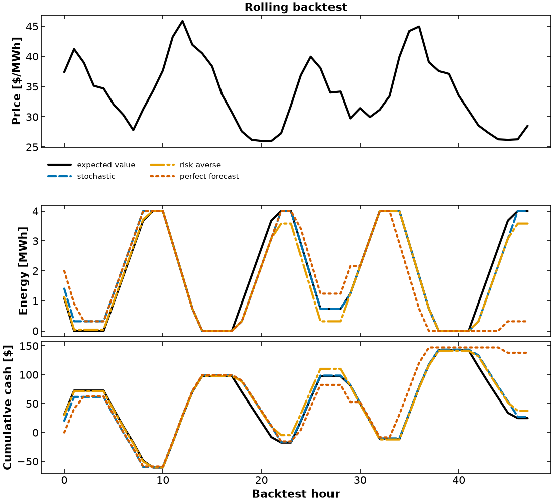

Interpret¶

Why can EVPI be positive when VSS is small?
How does scenario count change the metrics? Is the change monotone?
Does the risk-averse first action improve the lower tail, and what happens to mean profit?
Why is cash alone an unfair comparison when policies finish with different stored energy?
How much inventory-adjusted value separates the implementable policies from the oracle in this 48-hour sample?
Which assumption would you improve first: scenario construction, terminal valuation, battery degradation, market timing, or the two-stage information pattern?

One short backtest is evidence, not proof. A serious forecast comparison needs repeated out-of-sample windows and must charge every policy the same battery and market costs.

Interpretation limits and references¶

At seven equally weighted scenarios and confidence 0.9, the lower-tail CVaR is the minimum scenario profit (tail mass 0.1 is less than 1/7).
The comparison reports the exact lower-tail CVaR for this seven-scenario model, evaluated independently as the minimum scenario profit.
The rolling oracle is a benchmark with a finite horizon and terminal constraint, not a proven globally optimal policy for the entire backtest.
Birge and Louveaux (2011), 2nd ed., §§2.3–2.4, pp. 57–65; §§4.1–4.3, pp. 163–166.
Rockafellar and Uryasev (2002), Conditional Value-at-Risk for General Loss Distributions.