This notebook contains advanced topics for optimization under uncertainty.
Sample average approximation¶
Sample average approximation (SAA) replaces an expectation with a finite sample:
[ z_N = \min_{\mathbf{x}\in X}\frac{1}{N}\sum_{i=1}^{N}g(\mathbf{x},\boldsymbol{\xi}^i), \qquad \boldsymbol{\xi}^i \overset{\mathrm{iid}}{\sim} P. ]
A responsible SAA study separates:
a training sample used to choose (\mathbf{x}_N);
a larger, independent evaluation sample used to estimate out-of-sample performance; and
repeated samples used to measure solution variability.
One SAA solve is not a statistical guarantee. Sample size, random seed, and evaluation protocol are part of the model. A fixed candidate must be independent of assessment data. Within an assessment batch, candidate evaluation and re-optimization may deliberately share common random numbers; the paired gap is nonnegative. Independent replications estimate its uncertainty. See Mak, Morton and Wood (1999), and Bayraksan and Morton (2006).
Quadrature and sparse grids¶
Quadrature replaces an integral with a weighted sum,
[ \int f(x),dx \approx \sum_{i=1}^{n}\omega_i f(x_i). ]
Tensor-product quadrature grows exponentially with dimension. Sparse grids retain selected tensor-product points and can be effective for smooth, moderately dimensional integrands. They do not universally “defeat” dimensionality: performance depends on dimension, regularity, anisotropy, and the grid rule.
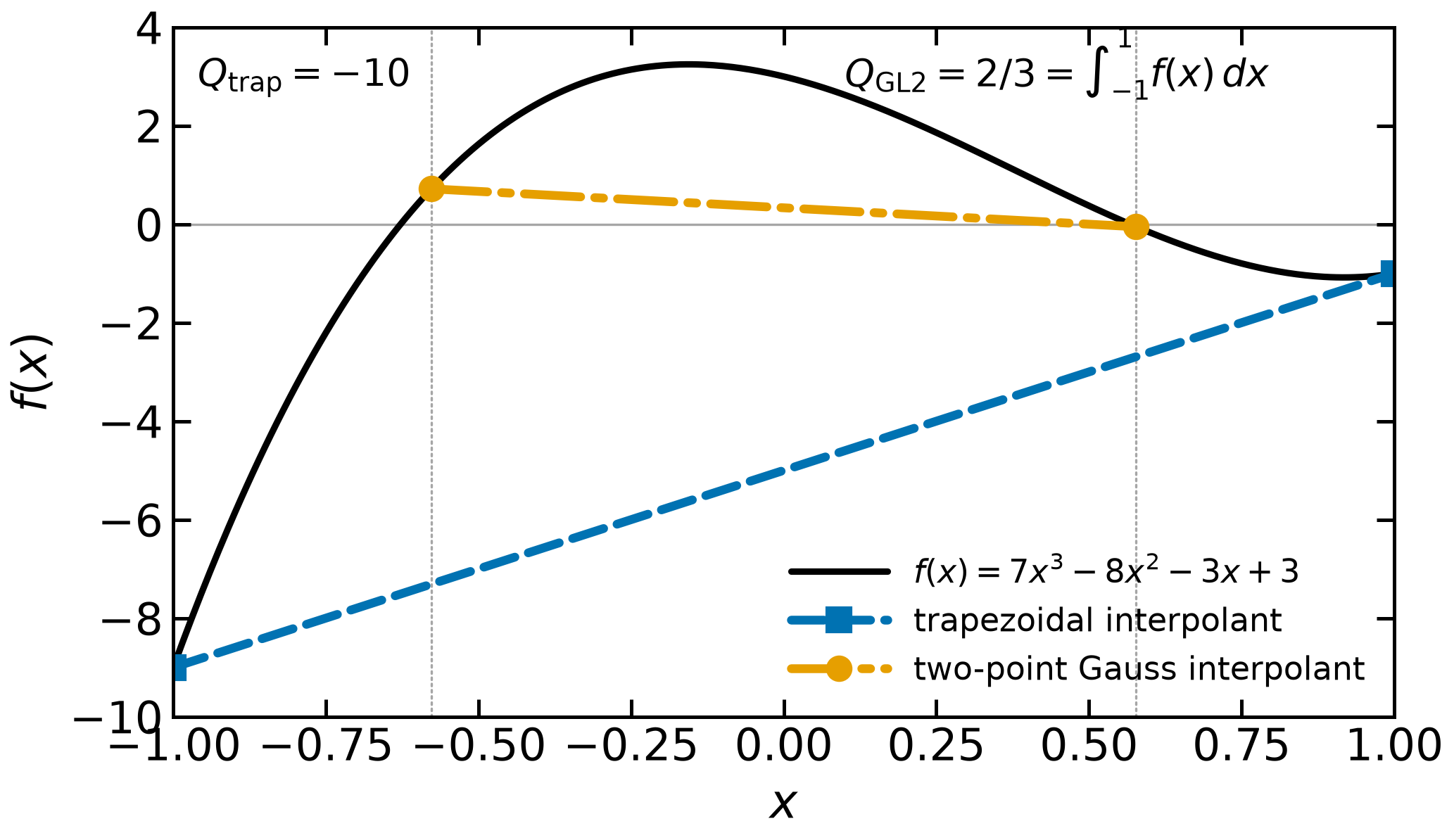
For (y(x)=7x^3-8x^2-3x+3) on ([-1,1]):
the exact integral is (2/3);
the endpoint trapezoid gives (-10); and
two-point Gauss--Legendre quadrature is exact because the integrand is cubic.
# Install course dependencies before importing Pyomo on Colab.
import sys

if "google.colab" in sys.modules:
    !wget "https://raw.githubusercontent.com/ndcbe/optimization/main/notebooks/helper.py"
    import helper

    helper.easy_install()
else:
    sys.path.insert(0, "../")
    import helper

helper.set_plotting_style()

import numpy as np

lower, upper = -1.0, 1.0


def integrand(x):
    return 7 * x**3 - 8 * x**2 - 3 * x + 3


# Odd powers integrate to zero; integrate -8*x**2 + 3 analytically.
exact = 2 / 3
trapezoid = (upper - lower) * (integrand(lower) + integrand(upper)) / 2
# Two nodes integrate polynomials through degree 3 exactly on [-1, 1].
nodes, weights = np.polynomial.legendre.leggauss(2)
gauss_legendre = sum(weights * integrand(nodes))

print(f"exact: {exact:.12f}")
print(f"trapezoid: {trapezoid:.12f}")
print(f"two-point Gauss--Legendre: {gauss_legendre:.12f}")
assert abs(gauss_legendre - exact) < 1e-12
exact: 0.666666666667
trapezoid: -10.000000000000
two-point Gauss--Legendre: 0.666666666667
Python implementations¶
NumPy supplies one-dimensional Gauss--Legendre nodes through numpy.polynomial.legendre.leggauss. The optional Tasmanian package provides several sparse-grid constructions.
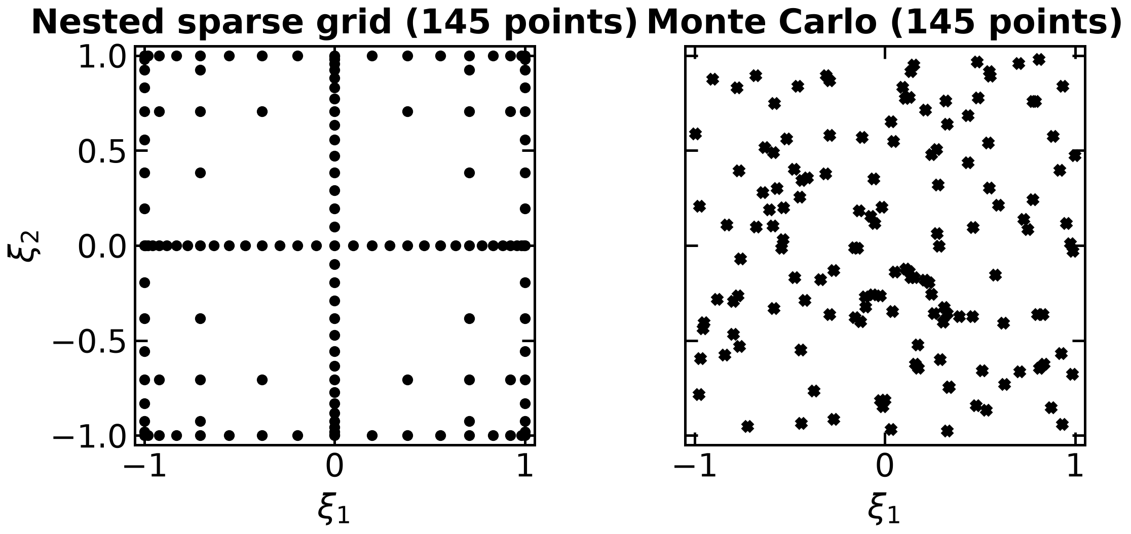
The course does not require Tasmanian. This notebook keeps the executable calculation dependency-light and uses the repository figure below for the sparse-grid concept.
The comparison uses the same number of points in two dimensions:
the sparse grid is a union of tensor products of nested Clenshaw--Curtis nodes; and
the Monte Carlo sample uses a fixed random seed.
Visual coverage alone does not establish accuracy. Compare integration error on an independent test problem.
A sample average approximation study¶
The section above is prose. This section is the computational companion: it builds an SAA problem from sampled scenarios, watches the solution move with the sample size, measures the optimistic bias of the sampled optimum, and computes a multiple-replication bound on the optimality gap.
The example is the farmer’s problem, the running example of the two stochastic programming lectures, taken from Birge and Louveaux, Introduction to Stochastic Programming, 2nd ed., §1.1a-b (pp. 4-8). The farmer allocates 500 acres among wheat, corn and sugar beets before the yield is known; purchases and sales are the recourse, chosen after the yield is observed. The recourse is real: a plan that looks good on average can force expensive wheat and corn purchases in a bad year.
One change makes it an SAA problem. The book’s Section 1.1b uses three equally likely yield scenarios, at , 0 and of the mean yields. A three-point distribution has nothing to approximate: the extensive form over all three points is the true problem. So this notebook uses a continuous law,
a single multiplier scaling all three crop yields. That is the book’s own next move: Section 1.1d (p. 11) takes each crop’s yield uniform on , chosen so the means still match Section 1.1b.
One difference from the book, and it changes the answer. Birge and Louveaux make the three crop yields independent, which lets the recourse separate crop by crop and even admits a closed-form . This notebook instead keeps the perfect correlation of the three-scenario model --- one common weather multiplier, as in Section 1.1b --- so the recourse does not separate. The practical consequence is that the expectation here is a one-dimensional integral, which is why the quadrature of the previous section can compute a reference answer below. Independent yields would make it three-dimensional, which is where the sparse-grid discussion starts to matter.
Cost convention. As in the lecture, the objective is minimized cost. Profit is the negative of cost, so the familiar appears below as a cost of .
Uniform yields are a modelling choice made for this demonstration, not a claim about agriculture. Nothing below depends on the choice except the numbers.
# The scenario structure is built with Pyomo Blocks: the stage 1 acreage lives on
# the model, and each sampled realization gets its own Block holding that
# sample's stage 2 purchases and sales. This is the same pattern used in
# "Stochastic Programming" (notebook 4/SP); the only difference is that the
# blocks are now indexed by a sample number instead of a named scenario, and
# there can be hundreds of them.
import numpy as np
import pyomo.environ as pyo
from pyomo.environ import units as u
from pyomo.util.check_units import assert_units_consistent
from scipy import stats

# Pyomo's unit library has acres and metric tons but no money, so declare one.
if not hasattr(u, "USD"):
    u.load_definitions_from_strings(["USD = [currency]"])

USD_PER_ACRE = u.USD / u.acre
USD_PER_TON = u.USD / u.metric_ton
TON_PER_ACRE = u.metric_ton / u.acre

# Birge & Louveaux, 2nd ed., Table 1, p. 5: mean yields [T/acre], planting costs
# [USD/acre], purchase and selling prices [USD/T], and the cattle feed
# requirements [T]. The 6000 T quota caps sales at the favorable beet price.
CROPS = ["WHEAT", "CORN", "BEETS"]
FEED_CROPS = ["WHEAT", "CORN"]
SALE_TYPES = ["WHEAT", "CORN", "BEETS_FAVORABLE", "BEETS_UNFAVORABLE"]

MEAN_YIELD = {"WHEAT": 2.5, "CORN": 3.0, "BEETS": 20.0}
PLANT_COST = {"WHEAT": 150.0, "CORN": 230.0, "BEETS": 260.0}
BUY_PRICE = {"WHEAT": 238.0, "CORN": 210.0}
SELL_PRICE = {
    "WHEAT": 170.0,
    "CORN": 150.0,
    "BEETS_FAVORABLE": 36.0,
    "BEETS_UNFAVORABLE": 10.0,
}
FEED_NEED = {"WHEAT": 200.0, "CORN": 240.0}
TOTAL_LAND = 500.0
BEET_QUOTA = 6000.0


def build_saa_model(multipliers, weights=None, check_units=False):
    """Extensive form over a list of yield multipliers, one Block per sample.

    Arguments:
        multipliers: yield multipliers, one per sample. Each scales all three
            mean yields.
        weights: probability weight of each sample. Defaults to 1/N, which is
            the sample average approximation. Passing quadrature weights
            instead turns the same builder into a deterministic integration
            rule, which is how the reference answer below is computed.
        check_units: run assert_units_consistent. Left off by default because
            it walks every constraint on every block, and these models are
            built hundreds of times; it is exercised on a small model below.

    Return:
        A Pyomo model whose objective is the weighted average cost in USD.
    """
    multipliers = np.asarray(multipliers, dtype=float)
    n = len(multipliers)
    if weights is None:
        weights = np.full(n, 1.0 / n)
    weights = np.asarray(weights, dtype=float)
    assert len(weights) == n, "one weight per sample"

    m = pyo.ConcreteModel()
    m.CROPS = pyo.Set(initialize=CROPS)
    m.FEED_CROPS = pyo.Set(initialize=FEED_CROPS)
    m.SALE_TYPES = pyo.Set(initialize=SALE_TYPES)
    m.SAMPLES = pyo.Set(initialize=range(n))

    # Stage 1: acres of each crop, chosen before any yield is observed [acre]
    m.acreage = pyo.Var(m.CROPS, domain=pyo.NonNegativeReals, units=u.acre)

    # Stage 1 cost [USD]
    m.planting_cost = sum(PLANT_COST[c] * USD_PER_ACRE * m.acreage[c] for c in CROPS)

    # Stage 1 constraint: the farm is 500 acres [acre]
    m.total_land_constraint = pyo.Constraint(
        expr=pyo.summation(m.acreage) <= TOTAL_LAND * u.acre
    )

    def scenario_block_rule(b, i):
        """Stage 2 for sample i. `b` is the block; `m` comes from the closure."""
        # Stage 2 decisions, made after the yield is observed [T]
        b.purchases = pyo.Var(
            m.FEED_CROPS, domain=pyo.NonNegativeReals, units=u.metric_ton
        )
        b.sales = pyo.Var(m.SALE_TYPES, domain=pyo.NonNegativeReals, units=u.metric_ton)

        b.purchase_cost = sum(
            BUY_PRICE[c] * USD_PER_TON * b.purchases[c] for c in FEED_CROPS
        )
        b.sales_revenue = sum(
            SELL_PRICE[s] * USD_PER_TON * b.sales[s] for s in SALE_TYPES
        )

        # Yields realized in this sample [T/acre]
        y = {c: MEAN_YIELD[c] * multipliers[i] for c in CROPS}

        # Feed requirements: grow it, buy it, or do not sell it [T]
        b.wheat_constraint = pyo.Constraint(
            expr=y["WHEAT"] * TON_PER_ACRE * m.acreage["WHEAT"]
            + b.purchases["WHEAT"]
            - b.sales["WHEAT"]
            >= FEED_NEED["WHEAT"] * u.metric_ton
        )
        b.corn_constraint = pyo.Constraint(
            expr=y["CORN"] * TON_PER_ACRE * m.acreage["CORN"]
            + b.purchases["CORN"]
            - b.sales["CORN"]
            >= FEED_NEED["CORN"] * u.metric_ton
        )
        # Beet sales cannot exceed beet production [T]
        b.beets_constraint = pyo.Constraint(
            expr=y["BEETS"] * TON_PER_ACRE * m.acreage["BEETS"]
            - b.sales["BEETS_FAVORABLE"]
            - b.sales["BEETS_UNFAVORABLE"]
            >= 0 * u.metric_ton
        )
        b.sales["BEETS_FAVORABLE"].setub(BEET_QUOTA)

    # One Block per sample: identical structure, different yield data
    m.scenarios = pyo.Block(m.SAMPLES, rule=scenario_block_rule)

    # Weighted average cost [USD]
    m.objective = pyo.Objective(
        expr=m.planting_cost
        + sum(
            weights[i] * (m.scenarios[i].purchase_cost - m.scenarios[i].sales_revenue)
            for i in range(n)
        ),
        sense=pyo.minimize,
    )

    if check_units:
        assert_units_consistent(m)
    return m


solver = pyo.SolverFactory("appsi_highs")
assert solver.available(), "HiGHS is required for this section"
print("HiGHS version:", solver.version())


def solve_model(m):
    """Solve and return the objective value, refusing anything but optimal."""
    results = solver.solve(m)
    assert pyo.check_optimal_termination(
        results
    ), f"Solve failed: termination={results.termination_condition}"
    return pyo.value(m.objective)


def first_stage(m):
    """The stage 1 acreage as a plain array, in the order of CROPS."""
    return np.array([pyo.value(m.acreage[c]) for c in CROPS])


def saa_optimum(multipliers, weights=None):
    """Solve the sampled problem: returns (objective, acreage)."""
    m = build_saa_model(multipliers, weights)
    return solve_model(m), first_stage(m)


def evaluate_candidate(acreage, multipliers, weights=None):
    """Weighted average cost of a FIXED stage 1 plan, recourse still optimized.

    Fixing the stage 1 variables on the same model is all that separates
    "choose a plan" from "grade a plan". Every block still solves its own
    recourse problem.
    """
    m = build_saa_model(multipliers, weights)
    for c, acres in zip(CROPS, acreage):
        m.acreage[c].fix(acres)
    return solve_model(m)
HiGHS version: (1, 15, 1)
Check the builder against the book before trusting it¶
Passing the three multipliers 0.8, 1.0, 1.2 with equal weights rebuilds exactly the book’s three-scenario extensive form, so its answer is known: Birge and Louveaux, Table 5, p. 8, report 170 acres of wheat, 80 of corn and 250 of sugar beets, for an expected profit of . Lecture 10 quotes the same number as .
# Birge & Louveaux Table 5, p. 8 -- the RP solution quoted in Lecture 10.
book_cost, book_acres = saa_optimum([0.8, 1.0, 1.2])
print(f"expected profit = ${-book_cost:,.0f}   (book: $108,390)")
print(
    "acres  wheat {:.1f}  corn {:.1f}  beets {:.1f}   (book: 170, 80, 250)".format(
        *book_acres
    )
)
assert abs(-book_cost - 108390.0) < 1.0
assert np.allclose(book_acres, [170.0, 80.0, 250.0], atol=1e-6)

# Exercise the unit declarations once, on a small model.
assert_units_consistent(build_saa_model([0.8, 1.0, 1.2], check_units=True))
print("units consistent")
expected profit = $108,390 (book: $108,390)
acres wheat 170.0 corn 80.0 beets 250.0 (book: 170, 80, 250)
units consistent
A reference answer, from the quadrature above¶
The uncertainty here is one-dimensional, so the true problem
can be solved to high
accuracy by deterministic integration rather than sampling: use a dense grid of
multipliers with trapezoid weights in place of the sampling weights. The
same build_saa_model does both; only the weights change.
This is a luxury, and it is the reason this notebook can check its own statistics. Real applications have no such reference — which is exactly why the sampled bounds of the following sections exist. Note also that is a piecewise-linear convex function of the multiplier (it is the value function of a linear program whose right-hand side moves linearly), so a high-order rule buys nothing at the kinks; refinement of a simple rule is the honest check.
def trapezoid_grid(n, lo=0.8, hi=1.2):
    """n-point trapezoid rule on [lo, hi] for a Uniform(lo, hi) expectation.

    The uniform density 1/(hi-lo) cancels the (hi-lo) in the quadrature
    weights, so the weights below sum to one and are directly comparable with
    the 1/N sampling weights.
    """
    nodes = np.linspace(lo, hi, n)
    weights = np.full(n, 1.0 / (n - 1))
    weights[0] = weights[-1] = 0.5 / (n - 1)
    return nodes, weights


print("grid      reference cost        wheat     corn    beets")
for n_grid in (201, 401, 801, 1601, 3201):
    nodes, weights = trapezoid_grid(n_grid)
    z_ref, x_ref = saa_optimum(nodes, weights)
    print(
        f"{n_grid:5d}   {z_ref:16,.4f}   {x_ref[0]:7.2f}  {x_ref[1]:6.2f}  {x_ref[2]:7.2f}"
    )

# Keep the finest grid as the reference for the rest of the section.
REF_NODES, REF_WEIGHTS = trapezoid_grid(3201)
Z_STAR, X_STAR = saa_optimum(REF_NODES, REF_WEIGHTS)
print(f"\nreference z* = {Z_STAR:,.2f} USD  (expected profit ${-Z_STAR:,.2f})")
grid reference cost wheat corn beets
201 -111,237.2935 135.56 85.11 279.33
401 -111,237.4344 135.82 85.11 279.07
801 -111,237.4383 135.87 85.06 279.07
1601 -111,237.4383 135.87 85.06 279.07
3201 -111,237.4405 135.84 85.06 279.10
reference z* = -111,237.44 USD (expected profit $111,237.44)
The last two refinements move the objective by a fraction of a dollar on a
quantity, so Z_STAR is treated below as exact. It is not the
book’s , and should not be: the distribution is different. A
continuous uniform yield spreads mass into the interior, where recourse is
cheaper than at the extremes.
How much does the solution move with the sample size?¶
One seeded draw per sample size. For each, solve the sampled problem, then
grade the resulting plan against the reference: q_ref is the plan’s true
expected cost and gap is how much worse than optimal it really is.
# One independent, seeded draw per sample size.
rng = np.random.default_rng(20260920)

print("    N       z_N          q_ref(x_N)     true gap     wheat    corn   beets")
sweep = []
for N in (5, 10, 25, 50, 100, 200, 500):
    xi = rng.uniform(0.8, 1.2, N)
    z_N, x_N = saa_optimum(xi)
    q_ref = evaluate_candidate(x_N, REF_NODES, REF_WEIGHTS)
    sweep.append((N, z_N, q_ref))
    print(
        f"{N:5d}  {z_N:12,.2f}  {q_ref:14,.2f}  {q_ref - Z_STAR:10,.2f}   "
        f"{x_N[0]:7.1f} {x_N[1]:6.1f} {x_N[2]:7.1f}"
    )
N z_N q_ref(x_N) true gap wheat corn beets
5 -98,025.42 -109,521.04 1,716.40 100.8 95.6 303.6
10 -110,484.82 -110,321.65 915.79 116.9 84.9 298.2
25 -101,488.46 -111,150.97 86.47 133.1 90.5 276.3
50 -116,479.50 -110,764.34 473.10 151.2 82.5 266.4
100 -108,751.64 -111,183.35 54.09 130.1 86.5 283.4
200 -114,580.54 -111,223.53 13.91 139.1 83.2 277.7
500 -111,873.95 -111,235.99 1.45 136.6 85.1 278.4
Two different things are moving in that table, and they should not be confused.
q_ref(x_N) - z\*is the quantity a decision maker cares about: the cost of using the sampled plan instead of the optimal one. It shrinks as grows, though not monotonically — this is one random draw per row, not an average.z_Nis the sampled objective, and it is not an estimate of anything the farmer receives. It wanders on both sides ofZ_STARby thousands of dollars, far more than the true gap ever is. A single sampled objective is not a performance number; reporting it as one is the mistake this section exists to prevent.
The sampled optimum is optimistically biased¶
Lecture 10 asks for the inequality directly. For any fixed feasible ,
In a minimization the sampled optimum is therefore too low on average: it looks better than anything achievable.
Measuring that bias directly, as , is hopeless at any affordable number of replications. The variance of is dominated by where the sample mean of happened to fall, and that noise is orders of magnitude larger than the bias. The fix is to subtract that noise off using the inequality itself, as a control variate: on each replication compute
both terms on the same sample. on every single replication — that is the first line of the display above, not a statistical claim — and is exactly the bias.
# Each replication solves the sampled problem and evaluates the reference plan
# on the SAME sample, so the shared sampling noise cancels in the difference.
rng_bias = np.random.default_rng(424242)
T_bias = 100
sizes = (5, 10, 20, 40, 80, 160)
bias_mean, bias_se = [], []

print(f"replications T = {T_bias}")
print("    N     mean D (bias)      std error    worst-case D      N x |bias|")
for N in sizes:
    D = np.empty(T_bias)
    for j in range(T_bias):
        xi = rng_bias.uniform(0.8, 1.2, N)
        D[j] = saa_optimum(xi)[0] - evaluate_candidate(X_STAR, xi)
    assert (D <= 0).all(), "the inequality above is pathwise, not on average"
    bias_mean.append(D.mean())
    bias_se.append(D.std(ddof=1) / np.sqrt(T_bias))
    print(
        f"{N:5d}  {D.mean():14,.2f}  {bias_se[-1]:12,.2f}  {D.max():14,.2f}  "
        f"{N * abs(D.mean()):14,.0f}"
    )
replications T = 100
N mean D (bias) std error worst-case D N x |bias|
5 -1,249.73 121.62 -36.07 6,249
10 -549.30 60.27 -11.22 5,493
20 -301.56 48.29 -8.59 6,031
40 -171.92 20.04 -1.28 6,877
80 -62.18 7.49 -0.12 4,974
160 -35.43 4.16 -0.96 5,669
The bias is negative at every sample size, as the inequality requires, it shrinks
as grows, and the last column is roughly constant — the bias here falls like
. The worst-case D column is the strongest statement in the table: the
largest of 100 values is still negative at every , because the inequality
holds on every draw and not merely in expectation.
Two cautions. The standard errors are on the estimated bias, not on itself, and they are small only because of the control variate. And here is the quadrature solution, not the exact optimizer; the grid refinement above bounds that substitution at well under a dollar, which is small compared with every bias in the table.
import matplotlib.pyplot as plt

fig, ax = plt.subplots(figsize=(5.5, 3.6))
ax.errorbar(
    sizes,
    [-b for b in bias_mean],
    yerr=bias_se,
    marker="o",
    linestyle="-",
    color="tab:blue",
    label=r"measured $|\mathbb{E}[z_N] - z^*|$",
)
reference = abs(bias_mean[0]) * sizes[0] / np.array(sizes, dtype=float)
ax.plot(
    sizes,
    reference,
    marker="s",
    linestyle="--",
    color="0.35",
    label=r"$1/N$ reference, anchored at $N=5$",
)
ax.set_xscale("log")
ax.set_yscale("log")
ax.set_xlabel("sample size $N$")
ax.set_ylabel("optimistic bias [USD]")
ax.set_title("Bias of the sampled optimum")
ax.legend(frameon=False, fontsize=8)
fig.tight_layout()
plt.show()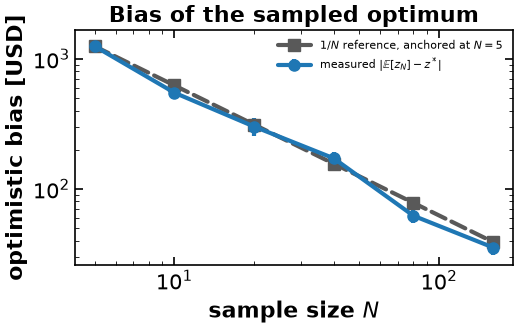
An optimality-gap certificate for one candidate plan¶
Now the estimator the lecture presents. Take a candidate from a deliberately small training sample, then assess it on fresh, independent batches. Within a batch, evaluate the candidate and re-optimize on the same realizations — common random numbers — so that
is a paired difference. The one-sided bound is .
The training sample is never reused here. Reusing it would report the training objective’s own optimism as if it were a bound.
# Training: a deliberately small sample, so the candidate is visibly imperfect.
rng_gap = np.random.default_rng(31415)
xi_train = rng_gap.uniform(0.8, 1.2, 20)
z_train, x_hat = saa_optimum(xi_train)
q_hat = evaluate_candidate(x_hat, REF_NODES, REF_WEIGHTS)
true_gap = q_hat - Z_STAR

print(
    f"candidate from N = 20: wheat {x_hat[0]:.1f}, corn {x_hat[1]:.1f}, "
    f"beets {x_hat[2]:.1f} acres"
)
print(f"training objective z_20      = {z_train:12,.2f}  (optimistic, not a bound)")
print(f"true expected cost q(x_hat)  = {q_hat:12,.2f}")
print(f"TRUE optimality gap          = {true_gap:12,.2f}  <- known only because")
print("                                               the reference exists\n")


def gap_bound(x_candidate, T, N, delta, seed):
    """Multiple-replication optimality-gap bound for a fixed candidate.

    Returns (G, bound). Each batch is fresh and independent of the others;
    within a batch the candidate evaluation and the re-optimization share the
    realizations, which is the paired (common random numbers) estimator.
    """
    rng_local = np.random.default_rng(seed)
    G = np.empty(T)
    for j in range(T):
        xi = rng_local.uniform(0.8, 1.2, N)
        G[j] = evaluate_candidate(x_candidate, xi) - saa_optimum(xi)[0]
    t_crit = stats.t.ppf(1.0 - delta, T - 1)  # ONE-sided critical value
    bound = G.mean() + t_crit * G.std(ddof=1) / np.sqrt(T)
    return G, bound


print("  T     N      G_bar       s_G     one-sided 95% bound    covers true gap?")
for T, N, seed in ((30, 50, 9001), (30, 200, 9002), (100, 200, 9003)):
    G, bound = gap_bound(x_hat, T=T, N=N, delta=0.05, seed=seed)
    assert (G >= -1e-6).all(), "paired gaps are nonnegative by construction"
    print(
        f"{T:4d} {N:5d}  {G.mean():9,.2f}  {G.std(ddof=1):8,.2f}  "
        f"{bound:18,.2f}    {'yes' if bound >= true_gap else 'NO'}"
    )
candidate from N = 20: wheat 133.5, corn 89.1, beets 277.4 acres
training objective z_20 = -107,210.81 (optimistic, not a bound)
true expected cost q(x_hat) = -111,193.97
TRUE optimality gap = 43.47 <- known only because
the reference exists
T N G_bar s_G one-sided 95% bound covers true gap?
30 50 138.27 96.77 168.29 yes
30 200 76.50 51.40 92.45 yes
100 200 71.88 48.45 79.92 yes
Read the table with the lecture’s cautions in hand.
The bound is not the gap. , and , so estimates something larger than the true gap. The bound is conservative on purpose, and the
G_barcolumn sitting well above the true gap is that conservatism, not an error. Raising shrinks it, because climbs toward ; raising only shrinks the -term.The -interval is approximate. It leans on a central limit theorem for the replicate mean. Lecture 10 records as a reported rule of thumb, not a guarantee for every distribution, and that is the status of the rows here.
These are not joint statements. The rows are separate nominal 95% one-sided bounds computed from separate seeds. Three of them do not certify anything at a joint 95% level, and neither does combining a candidate-value interval with a lower-bound interval.
covers true gap?is a check available only here. It is not part of the procedure and cannot be run in a real study. It is printed because a demonstration of a statistical bound should be checked against the answer when the answer happens to be known — and because one run agreeing proves nothing about coverage, which is a statement about many runs.
Everything above is seeded. Changing default_rng(...) in any cell is the
intended way to see how much of what you just read was the draw.
References¶
Birge and Louveaux (2011), Introduction to Stochastic Programming, 2nd ed., Springer. The farmer’s problem and its data are §1.1a–b, pp. 4–8 (data in Table 1, p. 5); the three-scenario solution used as a check is Table 5, p. 8; the continuous uniform-yield version is §1.1d, p. 11.
Mak, Morton and Wood (1999), Monte Carlo bounding techniques for determining solution quality in stochastic programs, DOI: Mak et al. (1999).
Bayraksan and Morton (2006), Assessing solution quality in stochastic programs, DOI: Bayraksan & Morton (2006).
NumPy Gauss–Legendre documentation: exactness through degree .
Tasmanian project documentation: optional sparse-grid software.
The two comparison figures are original course illustrations. The sparse-grid picture displays nodes, not quadrature weights or an error bound.
- Mak, W.-K., Morton, D. P., & Wood, R. K. (1999). Monte Carlo bounding techniques for determining solution quality in stochastic programs. Operations Research Letters, 24(1–2), 47–56. 10.1016/s0167-6377(98)00054-6
- Bayraksan, G., & Morton, D. P. (2006). Assessing solution quality in stochastic programs. Mathematical Programming, 108(2–3), 495–514. 10.1007/s10107-006-0720-x